OpenAI just released their new open-weight LLMs this week: gpt-oss-120b and gpt-oss-20b, their first open-weight models since GPT-2 in 2019. And yes, thanks to some clever optimizations, they can run locally (but more about this later).
This is the first time since GPT-2 that OpenAI has shared a large, fully open-weight model. Earlier GPT models showed how the transformer architecture scales. The 2022 ChatGPT release then made these models mainstream by demonstrating concrete usefulness for writing and knowledge (and later coding) tasks. Now they have shared some long-awaited weight model, and the architecture has some interesting details.
I spent the past few days reading through the code and technical reports to summarize the most interesting details. (Just days after, OpenAI also announced GPT-5, which I will briefly discuss in the context of the gpt-oss models at the end of this article.)
Below is a quick preview of what the article covers. For easier navigation, I recommend using the Table of Contents on the left of on the article page.
-
Model architecture comparisons with GPT-2
-
MXFP4 optimization to fit gpt-oss models onto single GPUs
-
Width versus depth trade-offs (gpt-oss vs Qwen3)
-
Attention bias and sinks
-
Benchmarks and comparisons with GPT-5
I hope you find it informative!
1. Model Architecture Overview
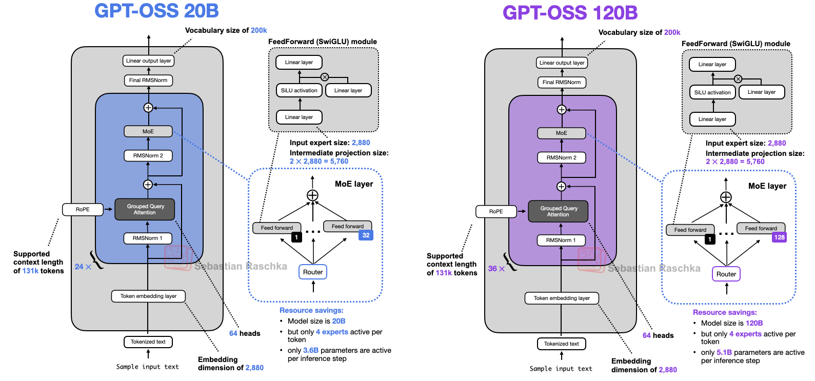
Before we discuss the architecture in more detail, let’s start with an overview of the two models, gpt-oss-20b and gpt-oss-120b, shown in Figure 1 below.
If you have looked at recent LLM architecture diagrams before, or read my previous Big Architecture Comparison article, you may notice that there is nothing novel or unusual at first glance. This is not surprising, since leading LLM developers tend to use the same base architecture and then apply smaller tweaks. This is pure speculation on my part, but I think this is because
-
There is significant rotation of employees between these labs.
-
We still have not found anything better than the transformer architecture. Even though state space models and text diffusion models exist, as far as I know no one has shown that they perform as well as transformers at this scale. (Most of the comparisons I found focus only on benchmark performance. It is still unclear how well the models handle real-world, multi-turn writing and coding tasks. At the time of writing, the highest-ranking non-purely-transformer-based model on the LM Arena is Jamba, which is a transformer–state space model hybrid, at rank 96.)
-
Most of the gains likely come from data and algorithm tweaks rather than from major architecture changes.
That being said, there are still many interesting aspects of their design choices. Some are shown in the figure above (while others are not, but we will discuss them later as well). In the rest of this article, I will highlight these features and compare them to other architectures, one at a time.
I should also note that I am not affiliated with OpenAI in any way. My information comes from reviewing the released model code and reading their technical reports. If you want to learn how to use these models locally, the best place to start is OpenAI’s official model hub pages:
The 20B model can run on a consumer GPU with up to 16 GB of RAM. The 120B model can run on a single H100 with 80 GB of RAM or newer hardware. I will return to this later, as there are some important caveats.
2. Coming From GPT-2
Before we jump into comparisons between gpt-oss and a more recent architecture, let’s hop into the time machine and take a side-by-side look at GPT-2 (Figure 2) to see just how far things have come.
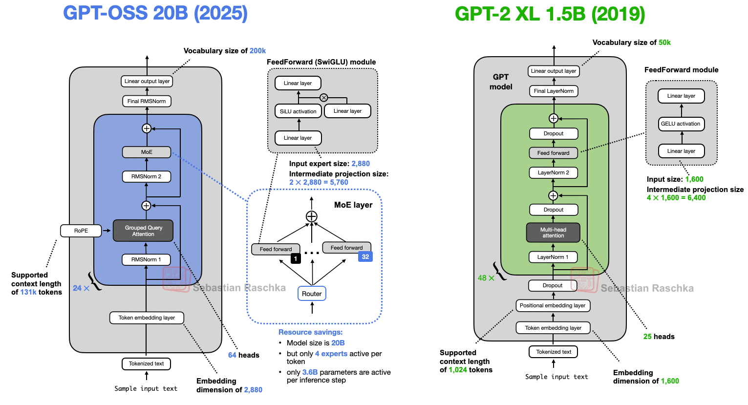
Both gpt-oss and GPT-2 are decoder-only LLMs built on the transformer architecture introduced in the Attention Is All You Need (2017) paper. Over the years, many details have evolved.
However, these changes are not unique to gpt-oss. And as we will see later, they appear in many other LLMs. Since I discussed many of these aspects in the previous Big Architecture Comparison article, I will try to keep each subsection brief and focused.
1.1 Removing Dropout
Dropout (2012) is a traditional technique to prevent overfitting by randomly “dropping out” (i.e., setting to zero) a fraction of the layer activations or attention scores (Figure 3) during training. However, dropout is rarely used in modern LLMs, and most models after GPT-2 have dropped it (no pun intended).
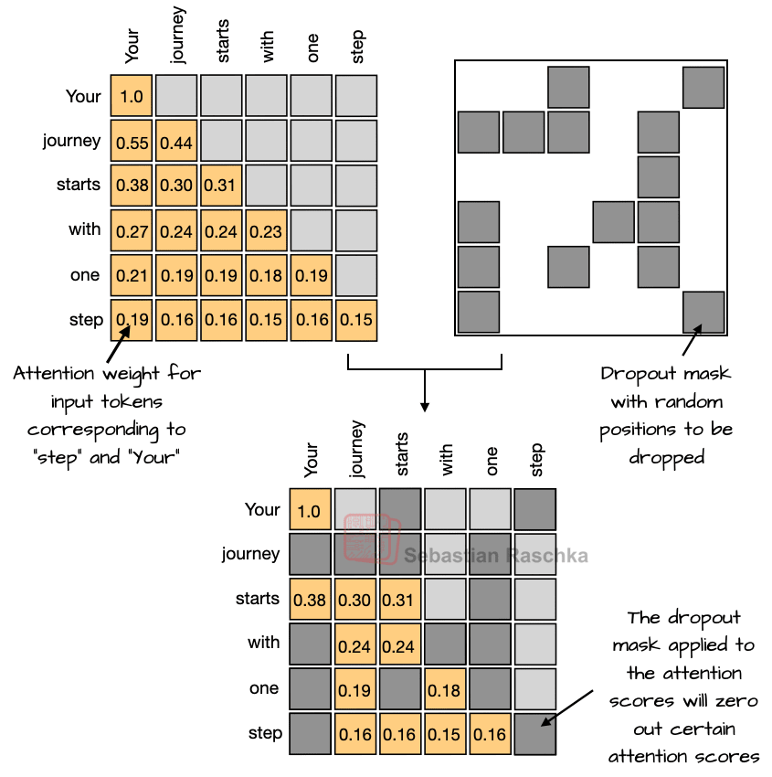
I assume that dropout was originally used in GPT-2 because it was inherited from the original transformer architecture. Researchers likely noticed that it does not really improve LLM performance (I observed the same in my small-scale GPT-2 replication runs). This is likely because LLMs are typically trained for only a single epoch over massive datasets, which is in contrast to the multi-hundred-epoch training regimes for which dropout was first introduced. So, since LLMs see each token only once during training, there is little risk of overfitting.
Interestingly, while Dropout is kind of ignored in LLM architecture design for many years, I found a 2025 research paper with small scale LLM experiments (Pythia 1.4B) that confirms that Dropout results in worse downstream performance in these single-epoch regimes.
1.2 RoPE Replaces Absolute Positional Embeddings
In transformer-based LLMs, positional encoding is necessary because of the attention mechanism. By default, attention treats the input tokens as if they have no order. In the original GPT architecture, absolute positional embeddings addressed this by adding a learned embedding vector for each position in the sequence (Figure 4), which is then added to the token embeddings.
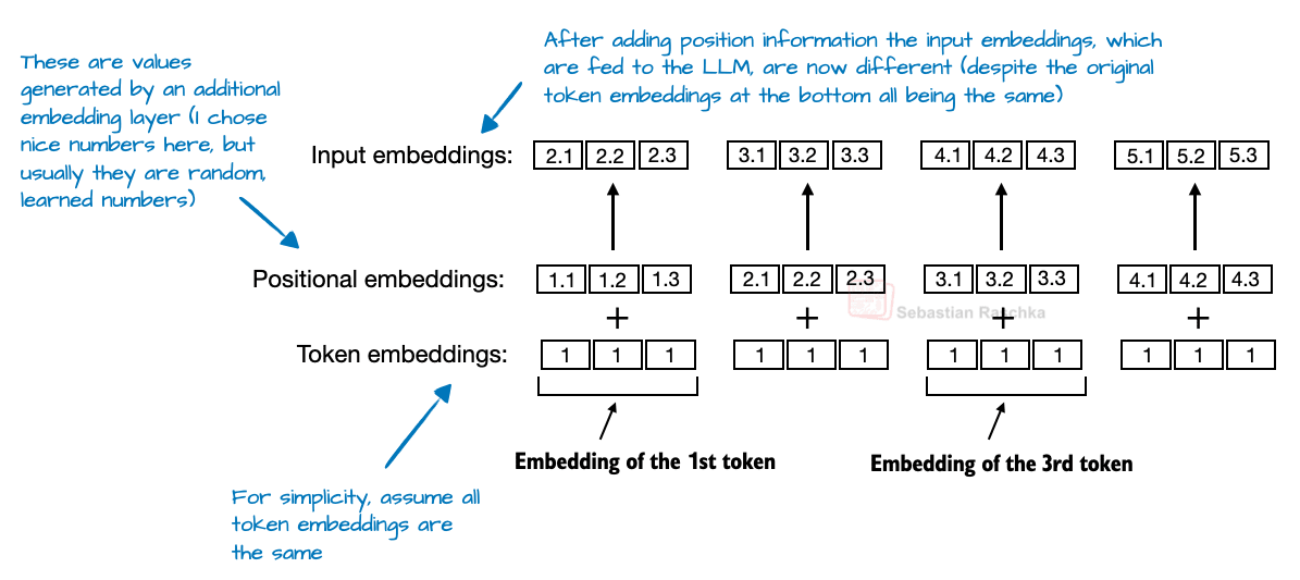
RoPE (Rotary Position Embedding) introduced a different approach: instead of adding position information as separate embeddings, it encodes position by rotating the query and key vectors in a way that depends on each token’s position. (RoPE is an elegant idea but also a bit of a tricky topic to explain. I plan to cover separately in more detail one day.)
While first introduced in 2021, RoPE became widely adopted with the release of the original Llama model in 2023 and has since become a staple in modern LLMs.
1.3 Swish/SwiGLU Replaces GELU
Early GPT architectures used GELU. Why now use Swish over GELU? Swish is considered computationally slightly cheaper, and in my opinion, that all there is to it. Depending on which paper you look at, you will find that one is slightly better than the other in terms of modeling performance. In my opinion, these small differences are probably within a standard error, and your mileage will vary based on hyperparameter sensitivity.
Activation functions used to be a hot topic of debate until the deep learning community largely settled on ReLU more than a decade ago. Since then, researchers have proposed and tried many ReLU-like variants with smoother curves, and GELU and Swish (Figure 5) are the ones that stuck.
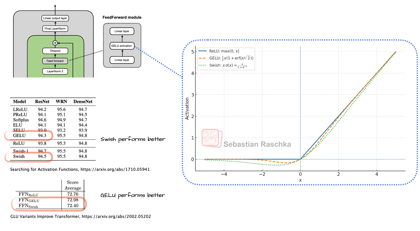
Early GPT architectures used GELU, which is defined as 0.5x * [1 + erf(x / sqrt(2))]. Here, erf (short for error function) is the integral of a Gaussian and it is computed using polynomial approximations of the Gaussian integral, which makes it more computationally expensive than simpler functions like the sigmoid used in Swish, where Swish is simply x * sigmoid(x).
In practice, Swish is computationally slightly cheaper than GELU, and that’s probably the main reason it replaced GELU in most newer models. Depending on which paper we look at, one might be somewhat better in terms of modeling performance. But I’d say these gains are often within standard error, and the winner will depend heavily on hyperparameter tuning.
Swish is used in most architectures today. However, GELU is not entirely forgotten; for example, Google’s Gemma models still use GELU.
What’s more notable, though, is that the feed forward module (a small multi-layer perceptron) is replaced by a gated “GLU” counterpart, where GLU stands for gated linear unit and was proposed in a 2020 paper. Concretely, the 2 fully connected layers are replaced by 3 fully connected layers that are used as shown in Figure 6 below.
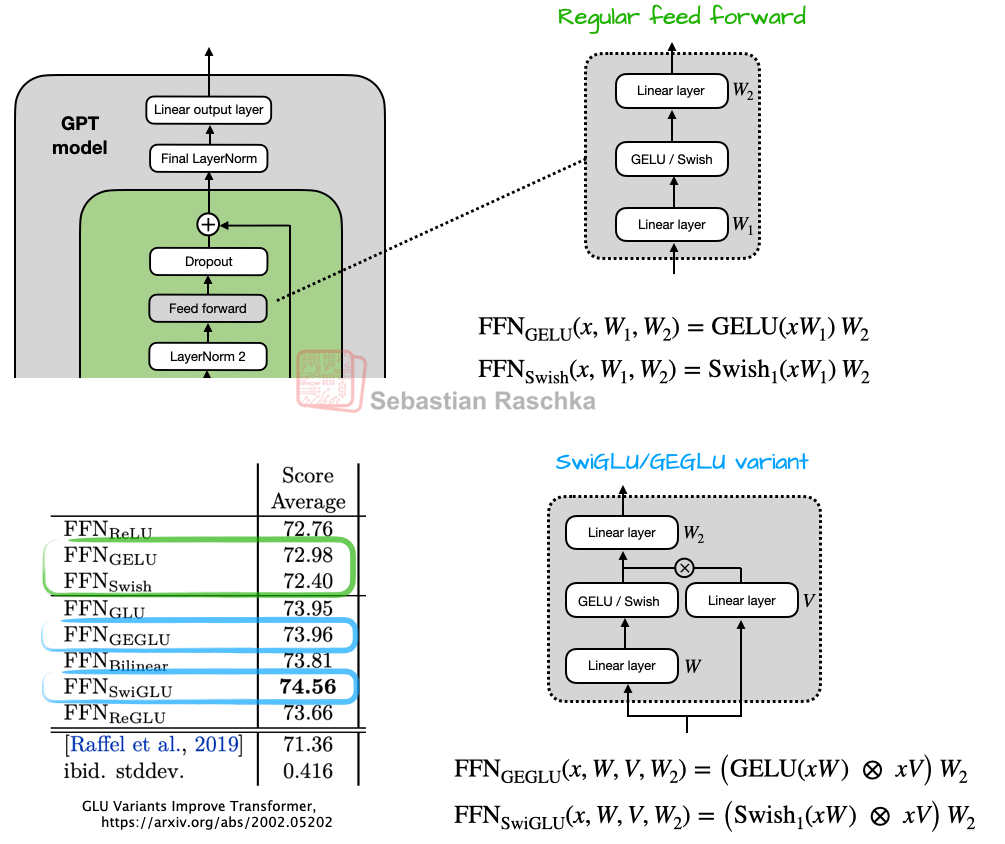
At first glance, it may appear that the GEGLU/SwiGLU variants may be better than the regular feed forward layers because there are simply more parameters due to the extra layer. But this is deceiving because in practice, the W and V weight layers in SwiGLU/GEGLU are usually chosen to be half the size each of the W_1 layer in a traditional feed forward layer.
To illustrate this better, consider the concrete code implementations of the regular and GLU variants:
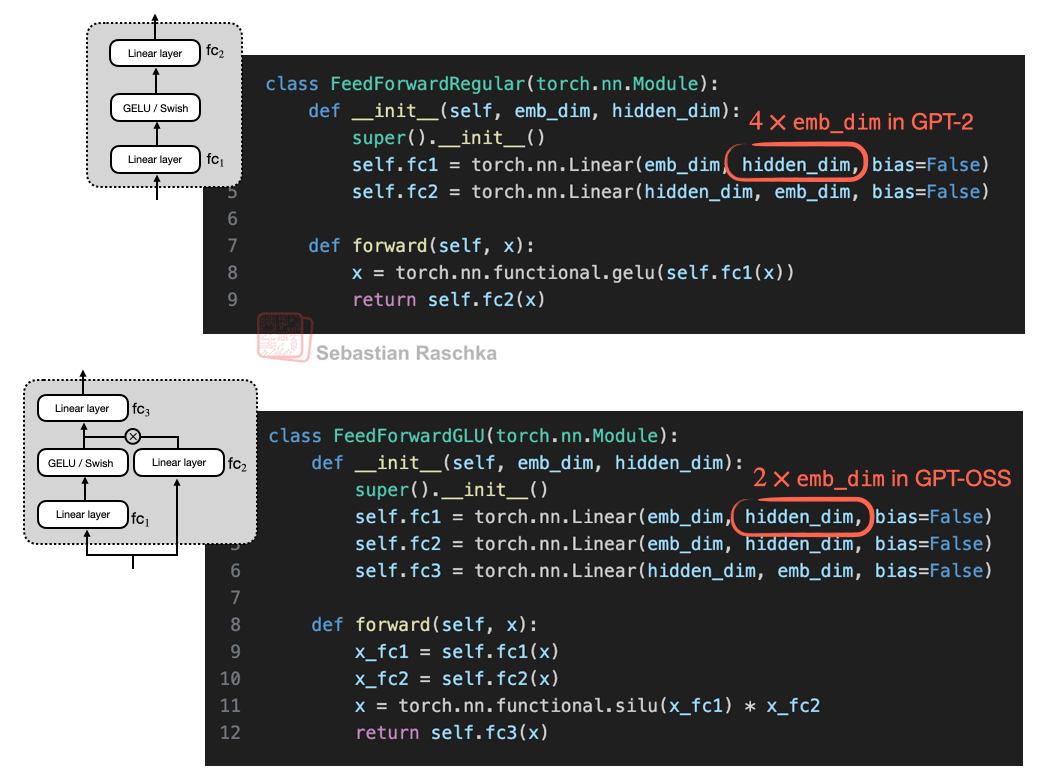
So, suppose we have an embedding dimension of 1024. In the regular feed forward case, this would then be
-
fc1: 1024 × 4096 = 4,194,304
-
fc2: 1024 × 4096 = 4,194,304
That is fc1 + fc2 = 8,388,608 parameters.
For the GLU variant, we have
-
fc1: 1024 × 2048 = 2,097,152
-
fc2: 1024 × 2048 = 2,097,152
-
fc3: 2048 × 1024 = 2,097,152
I.e., 3 × 2,097,152 = 6,291,456 weight parameters.
So, overall, using the GLU variants results in fewer parameters, and they perform better as well. The reason for this better performance is that these GLU variants provide an additional multiplicative interaction, which improves expressivity (the same reason deep & slim neural nets perform better than shallow & wide neural nets, provided they are trained well).
1.4 Mixture-of-Experts Replaces Single FeedForward Module
In addition to upgrading the feed forward module to a SwiGLU, as discussed in the previous section, gpt-oss replaces the single feed forward module with multiple feed forward modules, using only a subset for each token generation step. This approach is known as a Mixture-of-Experts (MoE) and illustrated in Figure 8 below.
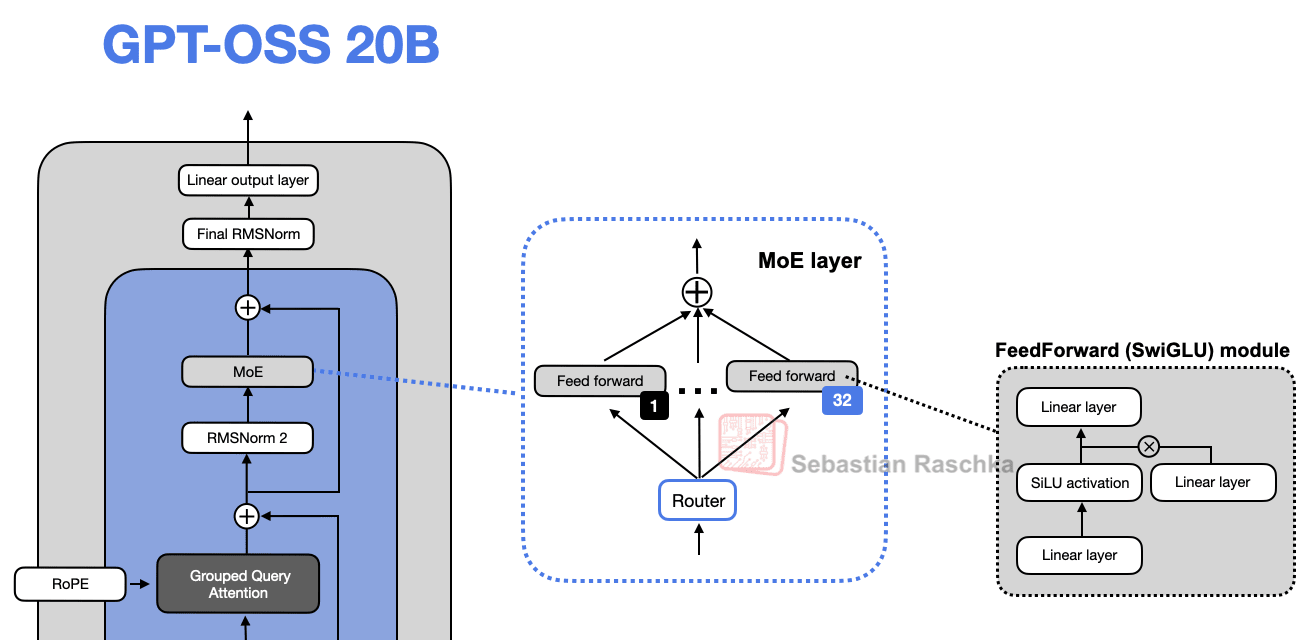
So, replacing a single feed forward module with multiple feed forward modules (as done in a MoE setup) substantially increases the model’s total parameter count. However, the key trick is that we don’t use (“activate”) all experts for every token. Instead, a router selects only a small subset of experts per token.
Because only a few experts are active at a time, MoE modules are often referred to as sparse, in contrast to dense modules that always use the full parameter set. However, the large total number of parameters via an MoE increases the capacity of the LLM, which means it can take up more knowledge during training. The sparsity keeps inference efficient, though, as we don’t use all the parameters at the same time.
(Fun fact: In most MoE models, expert weights account for more than 90% of the total model parameters.)
1.5 Grouped Query Attention Replaces Multi-Head Attention
As mentioned in my previous articles, Grouped Query Attention (GQA) has emerged in recent years as a more compute- and parameter-efficient alternative to Multi-Head Attention (MHA).
In MHA, each head has its own set of keys and values. GQA reduces memory usage by grouping multiple heads to share the same key and value projections.
For example, as shown in Figure 9, if there are 2 key–value groups and 4 attention heads, heads 1 and 2 might share one set of keys and values, while heads 3 and 4 share another. This grouping decreases the total number of key and value computations, leading to lower memory usage and improved efficiency — without noticeably affecting modeling performance, according to ablation studies.
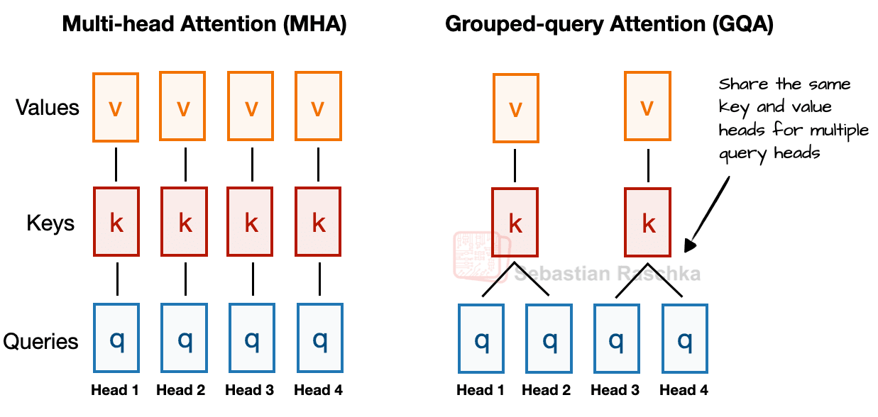
So, the core idea behind GQA is to reduce the number of key and value heads by sharing them across multiple query heads. This (1) lowers the model’s parameter count and (2) reduces the memory bandwidth usage for key and value tensors during inference since fewer keys and values need to be stored and retrieved from the KV cache.
(If you are curious how GQA looks in code, see my GPT-2 to Llama 3 conversion guide for a version without KV cache and my KV-cache variant here.)
While GQA is mainly a computational-efficiency workaround for MHA, ablation studies (such as those in the original GQA paper and the Llama 2 paper) show it performs comparably to standard MHA in terms of LLM modeling performance.
1.6 Sliding Window Attention
Sliding-window attention (Figure 10 below) was first introduced in the LongFormer paper (2020) and later popularized by Mistral. Interestingly, gpt-oss applies it in every second layer. You can think of it as a variation of multi-head attention, or in this case grouped query attention (GQA), where the attention context is restricted to a smaller window, reducing both memory usage and compute costs.
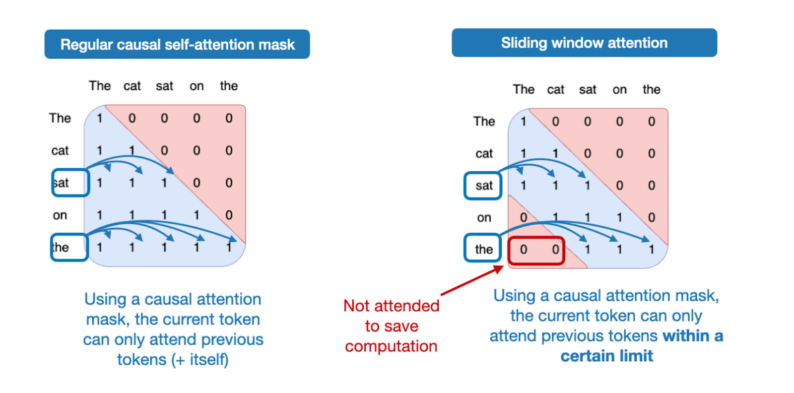
Concretely, gpt-oss alternates between GQA layers that attend to the full context and GQA layers with a sliding window limited to 128 tokens.
As I discussed in my previous article, Gemma 2 (2024) used a similar 1:1 ratio. Gemma 3 earlier this year went much further and shifted to a 5:1 ratio, which means only one full-attention layer for every five sliding-window (local) attention layers.
According to the Gemma ablation studies, sliding-window attention has minimal impact on modeling performance, as shown in the figure below. Note that the window size in Gemma 2 was 4096 tokens, which Gemma 3 reduced to 1024. In gpt-oss, the window is just 128 tokens, which is remarkably small.
And as a fun fact, the official announcement article notes that sliding-window attention was apparently already used in GPT-3:
The models use alternating dense and locally banded sparse attention patterns, similar to GPT-3
Who knew?
1.7 RMSNorm Replaces LayerNorm
Finally, the last small tweak, coming from GPT-2, is replacing LayerNorm (2016) by RMSNorm (2019), which has been a common trend in recent years.
Akin to swapping GELU with Swish and SwiGLU, RMSNorm is one of these smaller but sensible efficiency improvements. RMSNorm is similar to LayerNorm in its purpose to normalize layer activations, as shown in Figure 11 below.
You might recall that not too long ago, BatchNorm was the go-to choice for this task. It has since fallen out of favor, largely because it is harder to parallelize efficiently (due to the mean and variance batch statistics) and performs poorly with small batch sizes.
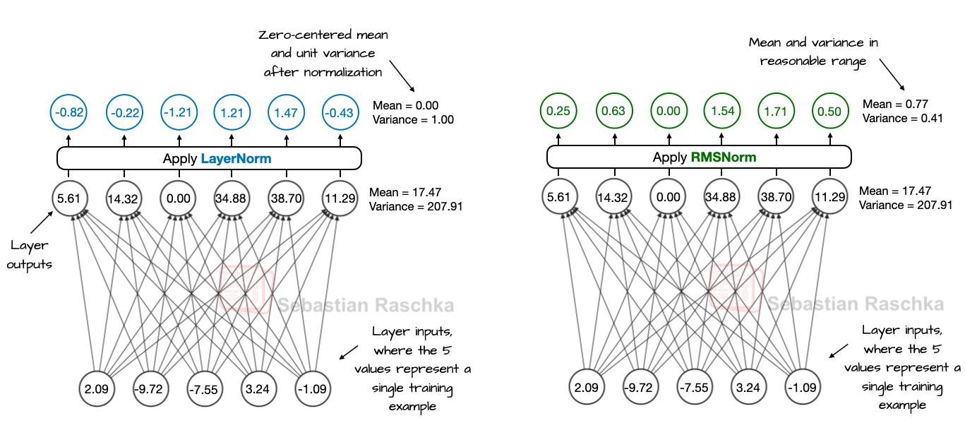
As we can see in Figure 11 above, both LayerNorm and RMSNorm scale the layer outputs to be in a reasonable range.
LayerNorm subtracts the mean and divides by the standard deviation such that the layer outputs have a zero mean and unit variance (variance of 1 and standard deviation of one).
RMSNorm divides the inputs by the root-mean-square. This doesn’t force zero mean and unit variance, but the mean and variance are in a reasonable range: -1 to 1 for the mean and 0 to 1 for the variance. In this particular example shown in Figure 11, the mean is 0.77 and the variance is 0.41.
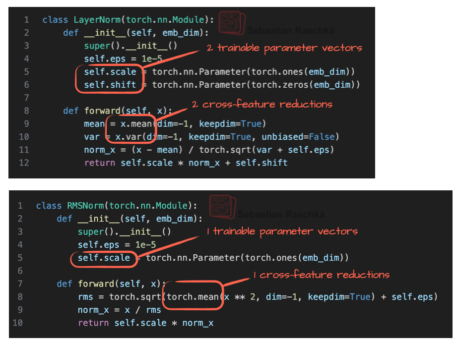
Both LayerNorm and RMSNorm stabilize activation scales and improve optimization, but RMSNorm is often preferred in large-scale LLMs because it is cheaper to compute. Unlike LayerNorm, RMSNorm has no bias (shift) term and reduces the expensive mean and variance computations to a single root-mean-square operation. This reduces the number of cross-feature reductions from two to one, which lowers communication overhead on GPUs and improving training efficiency.
Figure 12 shows what this looks like in code:
1.8 The GPT-2 Legacy
I still think that GPT-2 is an excellent beginner architecture when learning about LLMs. It’s simple enough to understand without getting lost in layers of optimization tricks, but still complex enough to give you a solid grasp of how modern transformer models work.
By starting with GPT-2, you can focus on the fundamentals (attention mechanisms, positional embeddings, normalization, and the overall training pipeline) without being overwhelmed by the extra features and tweaks found in newer architectures.
In fact, I think it’s worth the time to learn about and even implement GPT-2 first before trying to stack newer changes on top. You will not only have an easier time understanding those changes, but you will likely also appreciate them more, because you will get a better understanding of what limitations or problems they try to solve.
For instance, starting with my GPT-2 code I recently implemented the Qwen3 architecture from scratch, which is super similar to gpt-oss, which brings us to the next topic: Comparing gpt-oss to a more recent architecture.
3. Comparing gpt-oss To A Recent Architecture (Qwen3)
Now that we have walked through the evolution from GPT-2 to GPT OSS, we can take the next step and compare GPT OSS to a more recent architecture, Qwen3, which was released three months earlier in May 2025.
The reason I am selecting Qwen3 here is that it is among the top open-weight models as of the time of writing. Additionally, one of the Qwen3 MoE models is more or less directly comparable to GPT OSS due to its relatively similar overall size in terms of trainable parameters.
Figure 13 below compares gpt-oss-20b to a Qwen3 model of comparable size.
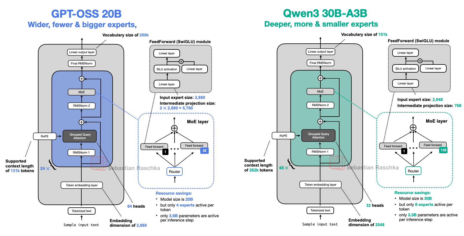
As we can see, gpt-oss 20B and Qwen3 30B-A3B are very similar in their architecture components. The primary difference here, aside from the dimensions, is that gpt-oss employs sliding window attention, as discussed earlier in section 1.6 (not shown in this figure), whereas Qwen3 does not.
Let’s walk through the noteworthy details one by one in the following subsections.
3.1 Width Versus Depth
If we look at the two models closely, we see that Qwen3 is a much deeper architecture with its 48 transformer blocks instead of 24 (Figure 14).
On the other hand, gpt-oss is a much wider architecture:
-
An embedding dimension of 2880 instead of 2048
-
An intermediate expert (feed forward) projection dimension of 5760 instead of 768
It’s also worth noting that gpt-oss uses twice as many attention heads, but this doesn’t directly increase the model’s width. The width is determined by the embedding dimension.
Does one approach offer advantages over the other given a fixed number of parameters? As a rule of thumb, deeper models have more flexibility but can be harder to train due to instability issues, due to exploding and vanishing gradients (which RMSNorm and shortcut connections aim to mitigate).
Wider architectures have the advantage of being faster during inference (with a higher tokens/second throughput) due to better parallelization at a higher memory cost.
When it comes to modeling performance, there’s unfortunately no good apples-to-apples comparison I am aware of (where parameter size and datasets are kept constant) except for an ablation study in the Gemma 2 paper (Table 9), which found that for a 9B parameter architecture, a wider setup is slightly better than a deeper setup. Across 4 benchmarks, the wider model achieved a 52.0 average score, and the deeper model achieved a 50.8 average score.
3.2 Few Large Versus Many Small Experts
As shown in Figure 14 above, it’s also noteworthy that gpt-oss has a surprisingly small number of experts (32 instead of 128), and only uses 4 instead of 8 active experts per token. However, each expert is much larger than the experts in Qwen3.
This is interesting because the recent trends and developments point towards more, smaller models as being beneficial. This change, at a constant total parameter size, is nicely illustrated in Figure 15 below from the DeepSeekMoE paper.
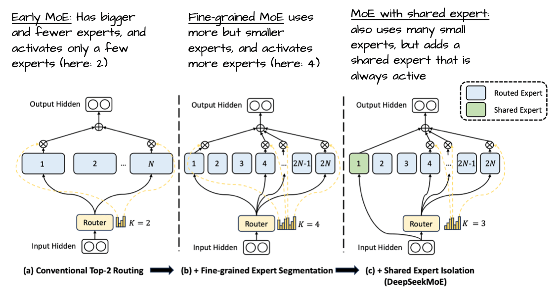
Notably, unlike DeepSeek’s models, neither gpt-oss nor Qwen3 uses shared experts, though.
To be fair, the small number of experts in gpt-oss could be a side effect of the 20B size. Looking at the 120B mode below, they indeed increased the number of experts (and transformer blocks) while keeping everything else fixed, as shown in Figure 16 below.
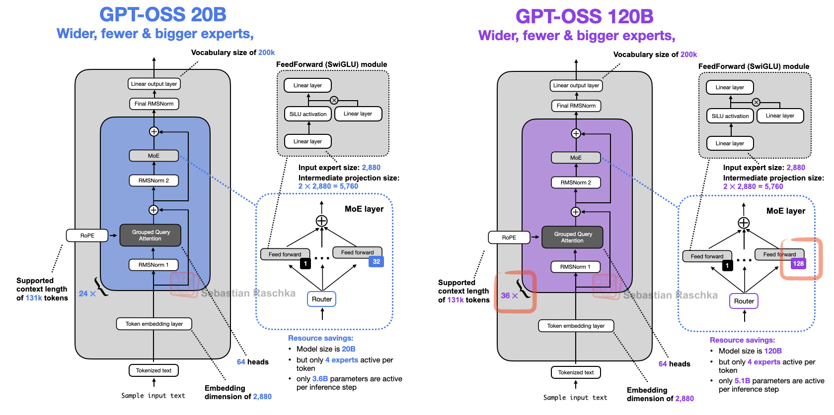
The boring explanation for the fact that the 20B and 120B models are so similar is probably that the 120B model was the main focus. And the easiest way to create a smaller model was to make it a bit shorter (fewer transformer blocks) and to reduce the number of experts, because that’s where most of the parameters are. However, one might speculate whether they started training the 120B model, and then chopped some of the transformer blocks and experts for continued pre-training (instead of starting from random weights).
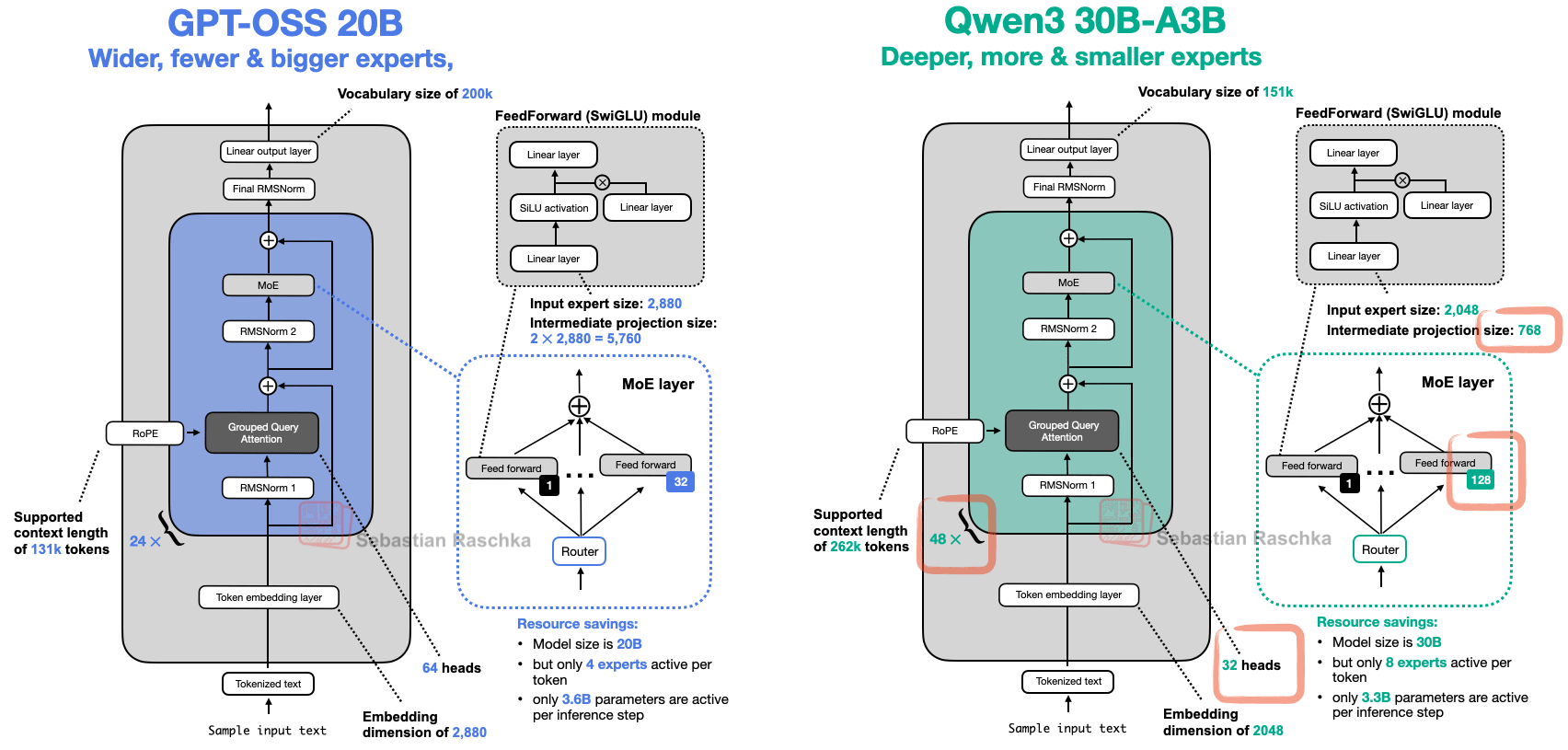
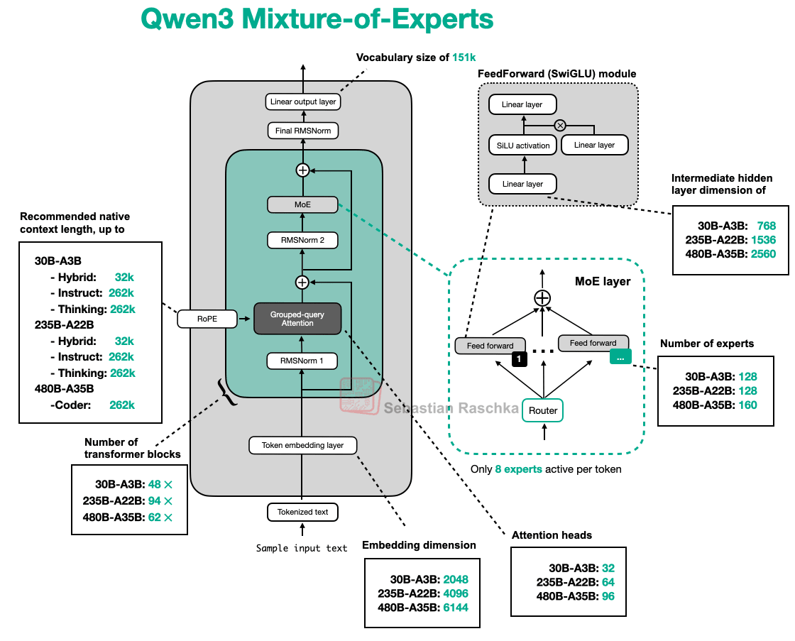
In any case, it’s because it’s quite unusual to only scale those two (transformer blocks and number of experts). For instance, when looking at Qwen3 MoE models of multiple sizes (Figure 17 below), they were scaled more proportionally to each other over many more aspects..
3.3 Attention Bias and Attention Sinks
Both gpt-oss and Qwen3 use grouped query attention. The main difference is that gpt-oss restricts the context size via sliding window attention in each second layer, as mentioned earlier.
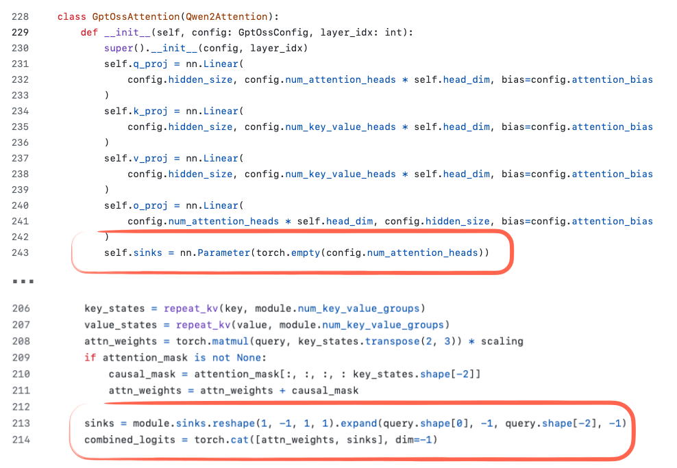
However, there’s one interesting detail that caught my eye. It seems that gpt-oss uses bias units for the attention weights, as shown in the figure below.
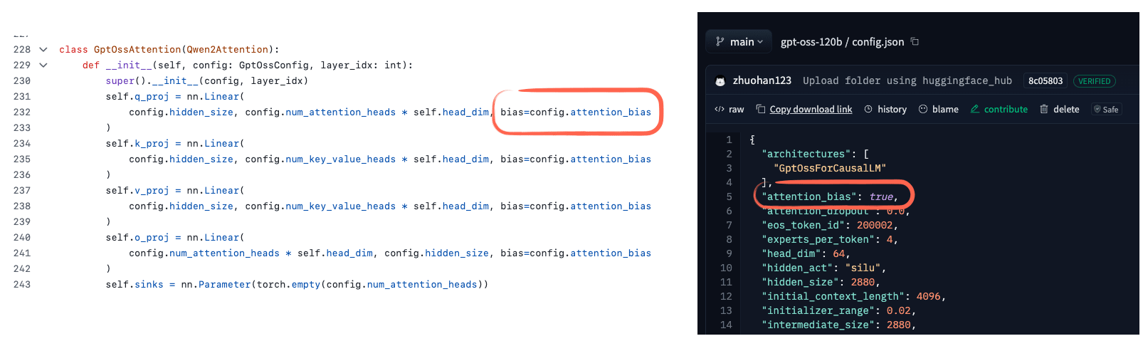
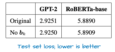
I haven’t seen these bias units being used since the GPT-2 days, and they are commonly regarded as redundant. Indeed, I found a recent paper that shows mathematically that this is at least true for the key transformation (k_proj). Furthermore, the empirical results show that there is little difference between with and without bias units (see Figure 19 below).
Another detail you may have noticed is the definition of sinks in the code screenshot in Figure 18. In general models, attention sinks are special “always-attended” tokens placed at the start of the sequence to stabilize attention, which is especially useful in long-context scenarios. I.e., if the context gets very long, this special attended token at the beginning is still attended to, and it can learn to store some generally useful information about the entire sequence. (I think it was originally proposed in the Efficient Streaming Language Models with Attention Sinks paper.)
In the gpt-oss implementation, attention sinks are not actual tokens in the input sequence. Instead, they are learned per-head bias logits that are appended to the attention scores (Figure 20). The goal is the same as with the above-mentioned attention sinks, but without modifying the tokenized inputs.
3.4 License
Lastly, and similar to Qwen3, the gpt-oss models are Apache 2.0 open-source license, which is great (it’s the same license that I prefer for my own open-source projects). This means that the models can be distilled into other models or used in commercial products without restriction.
Open-weight vs. open-source LLMs. This distinction has been debated for years, but it is worth clarifying to avoid confusion about this release and its artifacts. Some model developers release only the model weights and inference code (for example, Llama, Gemma, gpt-oss), while others (for example, OLMo) release everything including training code, datasets, and weights as true open source.
By that stricter definition, gpt-oss is an open-weight model (just like Qwen3) because it includes the weights and inference code but not the training code or datasets. However, the terminology is used inconsistently across the industry.
I assume the “oss” in “gpt-oss” stands for open source software; however, I am positively surprised that OpenAI itself clearly describes gpt-oss as an open-weight model in their official announcement article.
4 Other Interesting Tidbits
While the previous sections described how the architecture has evolved since GPT-2 and discussed its similarities to Qwen3 (and most other recent models), there are still a few additional but noteworthy details I have not mentioned, yet. These are points that did not fit neatly into the earlier sections but are still worth mentioning.
4.1 Training Overview
Unfortunately, there is not much information about the training set sizes and algorithms available. I added the most interesting puzzle pieces from the model card report (1) and announcement post (2) below:
The gpt-oss models were trained using our most advanced pre-training and post-training techniques […] (1)
[…] required 2.1million H100-hours to complete, with gpt-oss-20b needing almost 10x fewer. (1)
[…] including a supervised fine-tuning stage and a high-compute RL stage […] (2)
We trained the models on a mostly English, text-only dataset, with a focus on STEM, coding, and general knowledge. (2)
So, we know that the gpt-oss models are reasoning models. The training compute of 2.1 million H100 GPU hours is roughly on par with the 2.788 million H800 GPU hours that the ~5.6x larger DeepSeek V3 model was trained for. Unfortunately, there is no information about the Qwen3 training time available yet.
Interestingly, the GPT-oss training hour estimate includes both the supervised learning for instruction following and the reinforcement learning for reasoning, whereas DeepSeek V3 is just a pre-trained base model on top of which DeepSeek R1 was trained separately.
4.2 Reasoning Efforts
As mentioned in the previous section, the gpt-oss models are reasoning models. However, what’s particularly interesting is that they were trained so that users can easily control the degree of reasoning via inference time scaling.
Concretely, gpt-oss models can receive “Reasoning effort: low/medium/high” instructions as part of their system prompt, which directly affects the response length and accuracy, as shown in Figure 21.
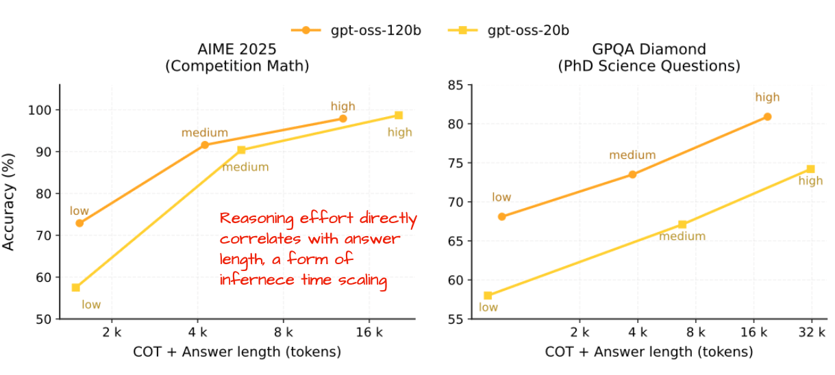
This level of adjustability is useful because it lets us balance cost, compute, and accuracy. For example, if the task is simple, such as answering a straightforward knowledge question or fixing a small typo, we can skip extended reasoning. This saves time and resources while avoiding unnecessarily long responses and verbose reasoning traces.
It is somewhat unfortunate that OpenAI did not release the base models prior to reinforcement learning-based reasoning training, unlike Qwen3 or OLMo. Base models are particularly valuable starting points for researchers working on reasoning methods (which is one reason I currently like working with Qwen3 Base). My guess is that OpenAI’s decision was driven more by industry and production use cases than by research considerations.
Note that the original Qwen3 models also have a toggle for enabling/disabling thinking (reasoning) modes (via a enable_thinking=True/False setting in the tokenizer that simply adds <think></think> tags to disable the reasoning behavior). However, the Qwen3 team updated their models in the last few weeks and moved away from the hybrid model towards dedicated Instruct/Thinking/Coder variants.
The reason was that the hybrid mode resulted in lower performance compared to the individual models:
After discussing with the community and reflecting on the matter, we have decided to abandon the hybrid thinking mode. We will now train the Instruct and Thinking models separately to achieve the best possible quality. Source
4.3 MXFP4 Optimization: A Small But Important Detail
One interesting surprise is that OpenAI released the gpt-oss models with an MXFP4 quantization scheme for the MoE experts.
Quantization formats used to be a niche topic, mostly relevant to mobile or embedded AI, but that’s changed with the push toward bigger models. In this case, the MXFP4 optimization allows the model to run on single GPU devices.
Here’s what that looks like in practice:
-
The large model (think 120B) fits on a single 80GB H100 or newer GPU. Not consumer hardware, but hey, it’s much cheaper to rent a 1-H100 machine than a multi-H100 machine. Plus, we don’t have to worry about distributing the model across GPUs and adding communication overhead. It’s really nice that AMD MI300X cards are supported from day 1 as well!
-
The smaller 20B model even fits into 16 GB of VRAM; the caveat is that it has to be a RTX 50-series GPU or newer to support MXFP4.
Note that the models will also run on older hardware but without MXFP4 support and will thus consume more RAM. Without MXFP4 optimization, the models in bfloat16 will consume more like 48 GB (gpt-oss-20b) and 240 GB (gpt-oss-120b).
4.4 Benchmarks
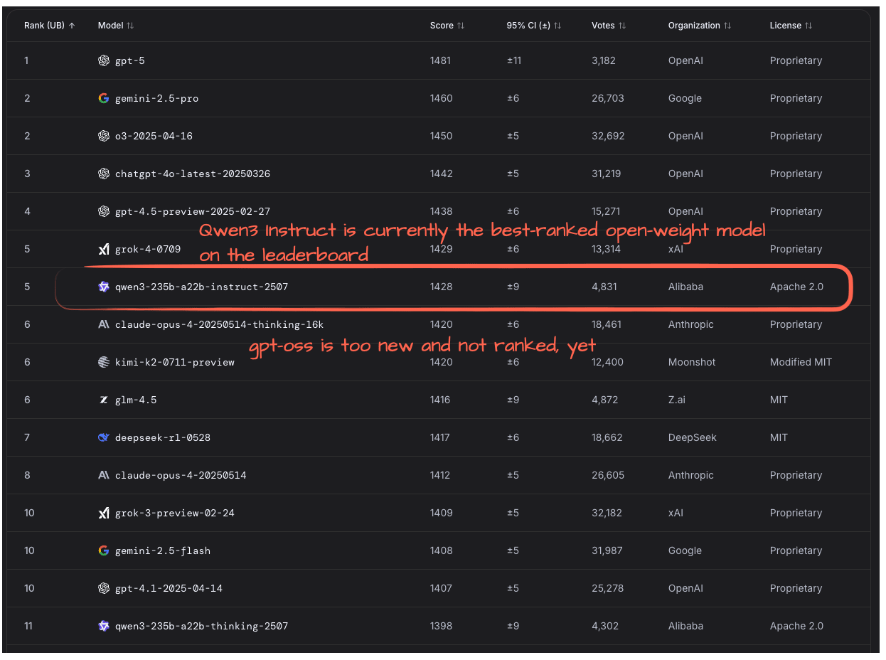
The models are still a bit too new for independent benchmarks. Checking the LM Arena leaderboard, I found that gpt-oss is not listed, yet. So, Qwen3-Instruct remains the top open-weight model, according to users on the LM Arena, for now (Figure 22).
Looking at a reasoning benchmarks provide in the gpt-oss announcement post, we can see that the gpt-ossmodels are on par with OpenAI’s proprietary models as well as Qwen3 (Figure 23).
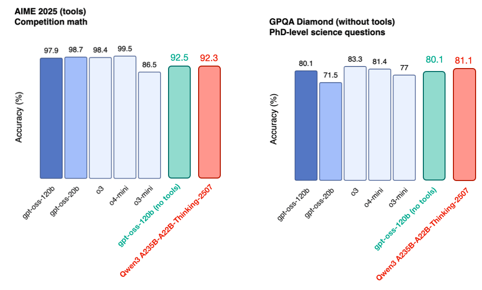
However, this should be caveated by the fact that gpt-oss-120b is almost half the size of the Qwen3 A235B-A22B-Thinking-2507 model and can run on a single GPU.
Benchmark performance, however, does not always reflect real-world usability. In my limited use over the past few days, I have found gpt-oss to be quite capable. That said, as others have observed, it does seem to have a relatively high tendency to hallucinate (a point also mentioned in its model card).
This may stem from its heavy training focus on reasoning tasks such as math, puzzles, and code, which could have led to some “general knowledge forgetting.” Still, because gpt-oss was designed with tool use in mind, this limitation may become less relevant over time. Tool integration in open-source LLMs is still in its early stages, but as it matures, I expect that we increasingly let models consult external sources (like search engines) when answering factual or knowledge-based queries.
If that happens, it could be sensible to prioritize reasoning capacity over memorization. This is much like in human learning in school (or in life in general), where problem-solving skills often matter more than memorizing facts.
5 gpt-oss and GPT-5
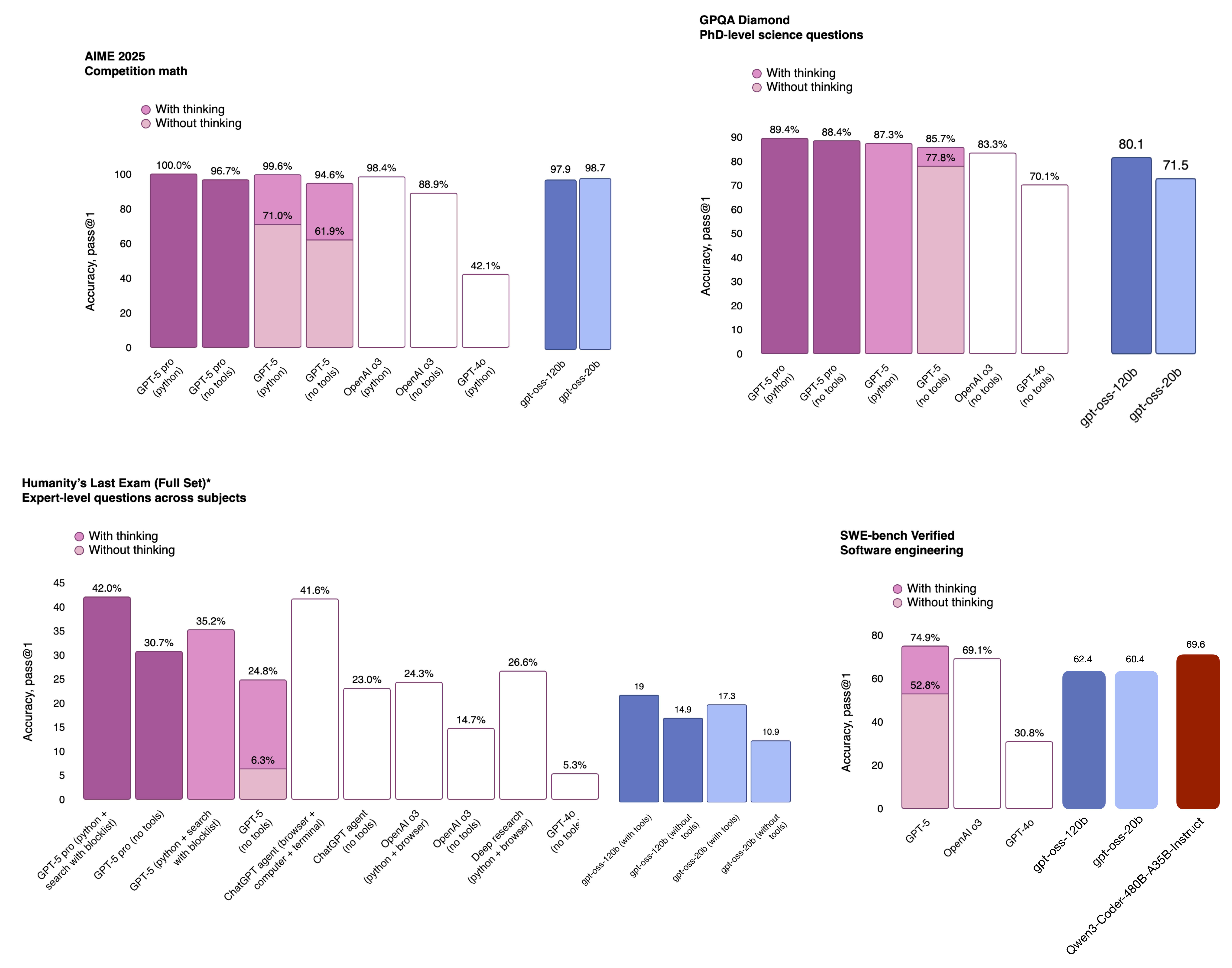
OpenAI had a busy week and released the long-awaited GPT-5 model shortly after gpt-oss. The GPT-5 release was interesting. And if there’s one thing I have to say here, it’s that I am really surprised by how good their open-source models really are compared to their best product offering in terms of benchmark performance (Figure 24).
All in all, even though some people called the release overhyped, I am glad that we have a new set of really strong open weight models that are not too far behind the best proprietary ones. Of course, benchmarks often do not accurately reflect real-world use, and it is still too early to tell based on the limited usage. But I think these are good times for people who like to work with open-weight and local (or privately hosted) models.
This magazine is a personal passion project, and your support helps keep it alive. If you would like to contribute, there are a few great ways:
-
Grab a copy of my book. Build a Large Language Model (From Scratch) walks you through building an LLM step by step, from tokenizer to training.
-
Check out the video course. There’s now a 17-hour video course based on the book, available from Manning. It follows the book closely, section by section, and works well both as a standalone or as a code-along resource. The video course is ad-free (unlike the YouTube version) and has a cleaner, more structured format. It also contains 5 additional hours of pre-requisite video material created by Abhinav Kimothi.
-
Subscribe. A paid subscription helps to make my writing sustainable and gives you access to additional contents.
Thanks for reading, and for helping support independent research!