After a short family break, I am excited to be back and catching up on a busy few weeks of open-weight LLM releases. The thing that stood out to me is how much newer architectures are focused on long-context efficiency.

As reasoning models and agent workflows keep more tokens around (for longer), KV-cache size, memory traffic, and attention cost quickly become the main constraints, and LLM developers are adding a growing number of architecture tricks to reduce those costs.

The main examples I want to look at are KV sharing and per-layer embeddings in Gemma 4, layer-wise attention budgeting in Laguna XS.2, compressed convolutional attention in ZAYA1-8B, and mHC plus compressed attention in DeepSeek V4.

Most of these changes look like small tweaks in my architecture diagrams, but some of them are quite intricate design changes that are worth a more detailed discussion.

Note that this article is about architecture designs, so I will mostly skip dataset mixtures, training schedules, post-training details, RL recipes, benchmark tables, and product comparisons. Even with that narrower scope, there is a lot to cover. And, like always, the article turned out longer than I expected, so I will keep the focus on what changes inside the transformer block, residual stream, KV cache, or attention computation.

Please also note that I am only covering those topics that are interesting (new) design choices and that I haven’t covered elsewhere, yet. This list includes:

1. KV sharing and per-layer embeddings in Gemma 4

2. Compressed convolutional attention in ZAYA1

3. Attention budgeting in Laguna XS.2

4. mHC and compressed attention in DeepSeek V4

Previous Topics

Before getting into the new parts, here are the two previous articles I will refer back to. The first one gives a broader architecture background on recent MoE models, routed experts, active parameters, and model-size comparisons. The second one covers the attention background that comes up repeatedly below, including MHA, MQA, GQA, MLA, sliding-window attention, sparse attention, and hybrid attention designs.

I also turned several of these explanations into short, standalone tutorial pages in the LLM Architecture Gallery. For example, readers can find compact explainers for GQA, MLA, sliding-window attention, DeepSeek Sparse Attention, MoE routing, and other concepts linked from the corresponding model cards and concept labels.

1. Reusing KV Tensors Across Layers to Shrink the Cache (Gemma 4)

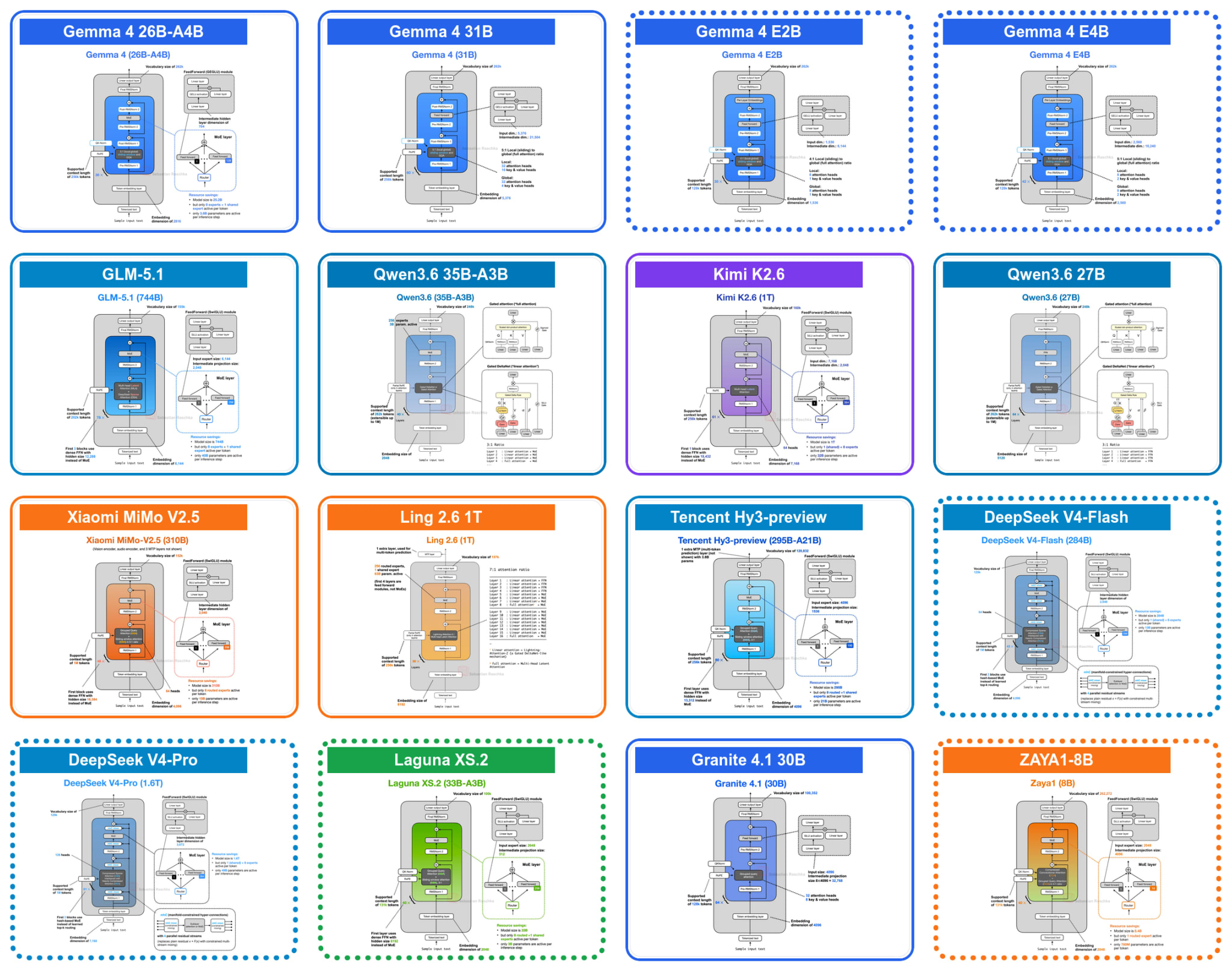
For this tour of architecture advances and tweaks, we will go back to the beginning of April when Google released their new open-weight Gemma 4 suite of models. They come in 3 broad categories:

• the Gemma 4 E2B and E4B models for mobile and small, local (embedded) devices (aka IoT),

• the Gemma 4 26B mixture-of-experts (MoE) model, optimized for efficient local inference,

• and the Gemma 4 31B dense model, for maximum quality and more convenient post-training (since MoEs are trickier to work with)

The first small architecture tweak in the E2B and E4B variants is that they adopt a shared KV cache scheme, where later layers reuse key-value states from earlier layers to reduce long-context memory and compute.

This KV-sharing was not invented by Gemma 4. For instance, see Brandon et al., “Reducing Transformer Key-Value Cache Size with Cross-Layer Attention” (NeurIPS 2024). But it’s the first popular architecture where I saw this concept applied. (Cross-layer attention is not to be confused with cross-attention.)

Before explaining KV-sharing further, let’s briefly talk about the motivation. As I wrote and talked about in recent months, one of the main recent themes in LLM architecture design is KV cache size reduction. In turn, the motivation behind KV cache size reduction is to reduce the required memory, which allows us to work with longer contexts, which is especially relevant in the age of reasoning models and agents. For more background on KV caching, see my “Understanding and Coding the KV Cache in LLMs from Scratch” article:

Practically all of the popular attention variants I described in my previous A Visual Guide to Attention Variants in Modern LLMs article are designed to reduce the KV cache size:

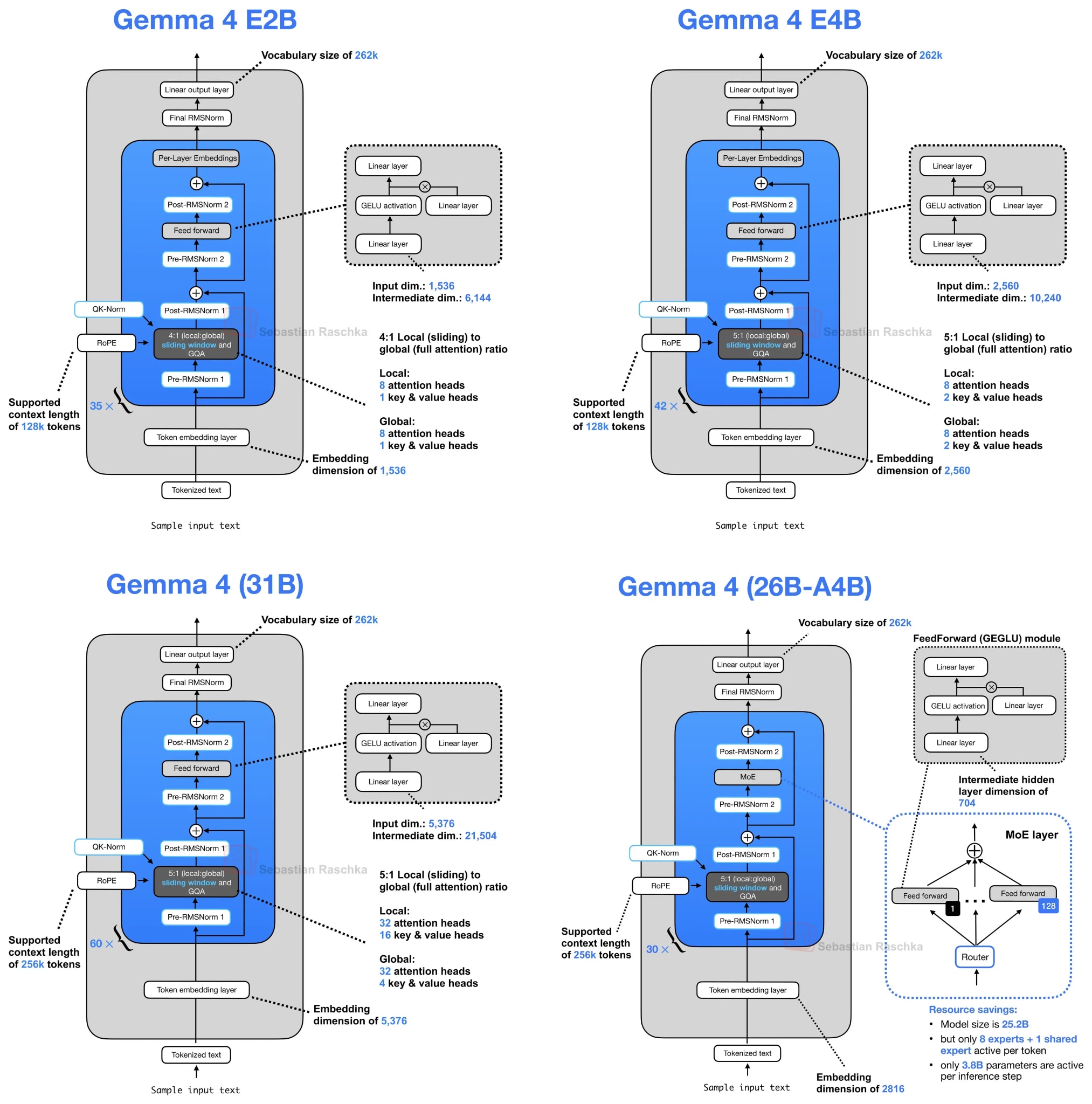
To pick a classic example (that Gemma 4 still uses): Grouped Query Attention (GQA) already shares key-value (KV) heads across different query heads to reduce the KV cache size, as illustrated in the figure below.

As mentioned before, Gemma 4 uses GQA. However, in addition to the KV sharing among queries as part of GQA, Gemma 4 also shares KV projections across different layers instead of computing it as part of the attention module in each layer. This KV-sharing scheme, also called cross-layer attention, is illustrated in the figure below.

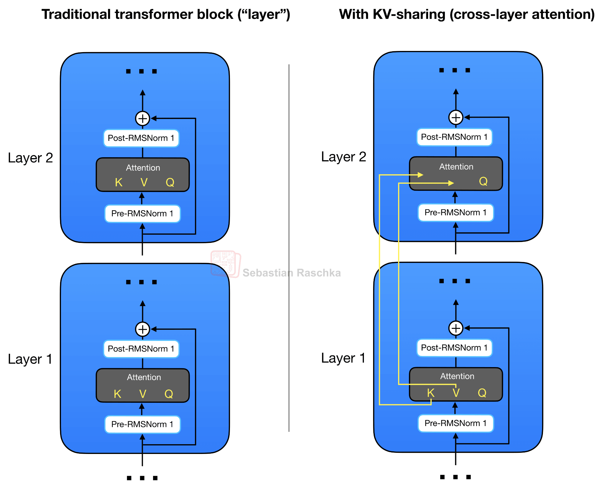
As briefly hinted at in the architecture overview in Figure 2, Gemma 4 E2B uses regular GQA and sliding window attention in a 4:1 pattern. (More precisely, Gemma 4 E2B uses MQA, which is the one-KV-head special case of GQA).

In the case of GQA (or MQA), the KV-sharing works like this. Later layers no longer compute their own key and value projections but reuse the KV tensors from the most recent earlier non-shared layer of the same attention type. In other words, sliding-window layers share KV with a previous sliding-window layer. Full-attention layers share KV with a previous full-attention layer. The layers still compute their own query projections, so each layer can form its own attention pattern, but the expensive and memory-heavy KV cache is reused across several layers.

For example, Gemma 4 E2B has 35 transformer layers, but only the first 15 compute their own KV projections; the final 20 layers reuse KV tensors from the most recent earlier non-shared layer of the same attention type. Similarly, Gemma 4 E4B has 42 layers, with 24 layers computing their own KV and the final 18 layers sharing them.

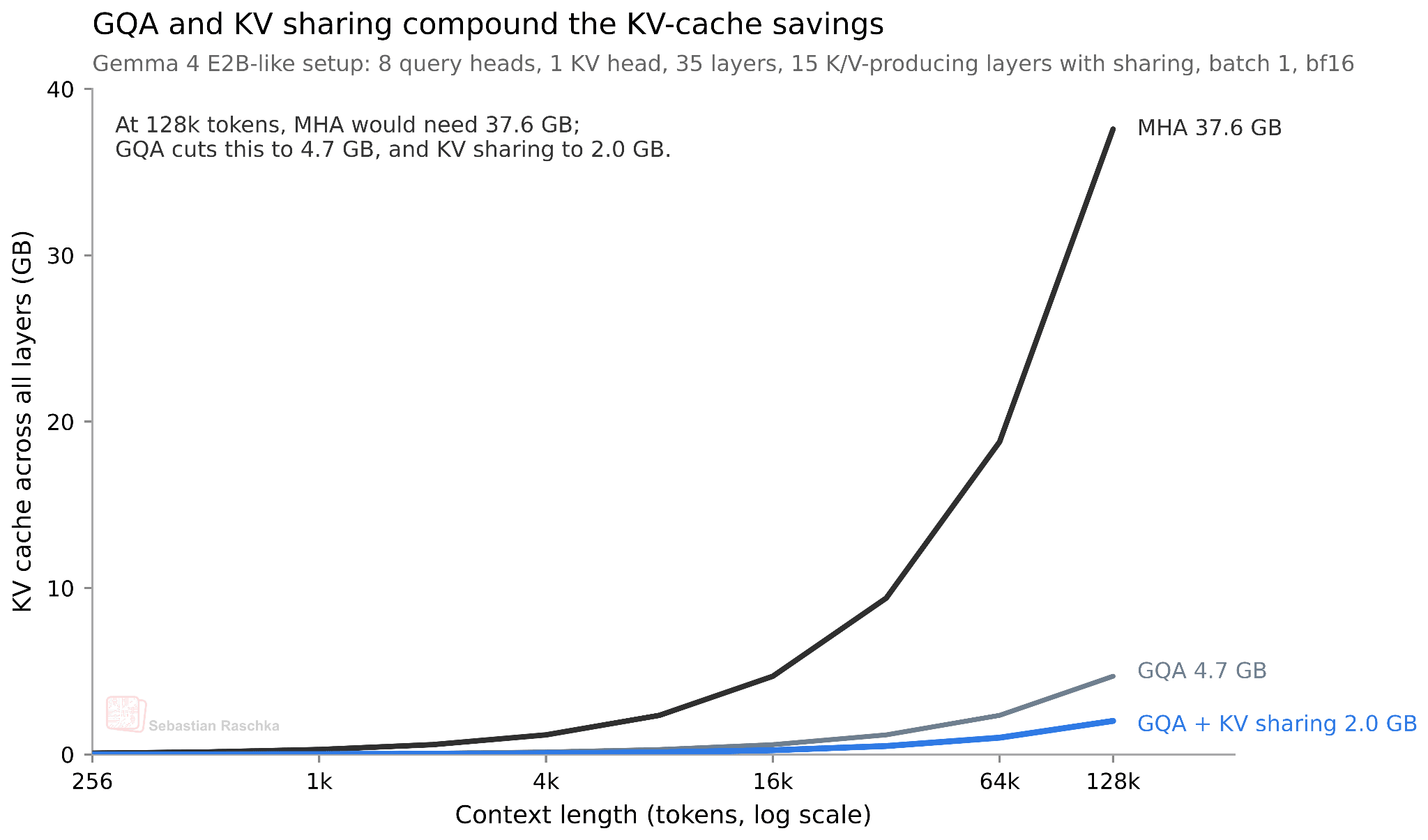
How much does this actually save? Since we share roughly half of the KVs across layers, we save approximately half of the KV cache size. For the smallest E2B model, this results in a 2.7 GB saving (at bfloat16 precision) in long 128K contexts, as shown below. (For the E4B variant, this saves about 6 GB at 128K.)

The downside of KV-sharing is, of course, that it’s an “approximation” of the real thing. Or, more precisely, it reduces model capacity. However, according to the cross-layer attention paper, the impact can be minimal (for small models that were tested).

2. Per-Layer Embeddings and “Effective” Size (Gemma 4 E2B/E4B)

The Gemma 4 E2B and E4B variants include a second efficiency-oriented design choice called per-layer embeddings (PLE). This is separate from the KV-sharing scheme above.

KV sharing reduces the KV cache. PLE is instead about parameter efficiency, where it lets the small Gemma 4 models use more token-specific information without making the main transformer stack as expensive as a dense model with the same total parameter count.

For instance, the “E” in Gemma 4 E2B and E4B stands for “effective”. Concretely, Gemma 4 E2B is listed as 2.3B effective parameters, or 5.1B parameters when the embeddings are counted. (Similarly, Gemma 4 E4B is listed as 4.5B effective parameters, or 8B parameters with embeddings).

In short, in the “E” models, the main transformer-stack compute is closer to the smaller number, while the larger number includes the additional embedding-table layers. (For an illustration of how embedding layers work, see my “Understanding the Difference Between Embedding Layers and Linear Layers” code notebook.)

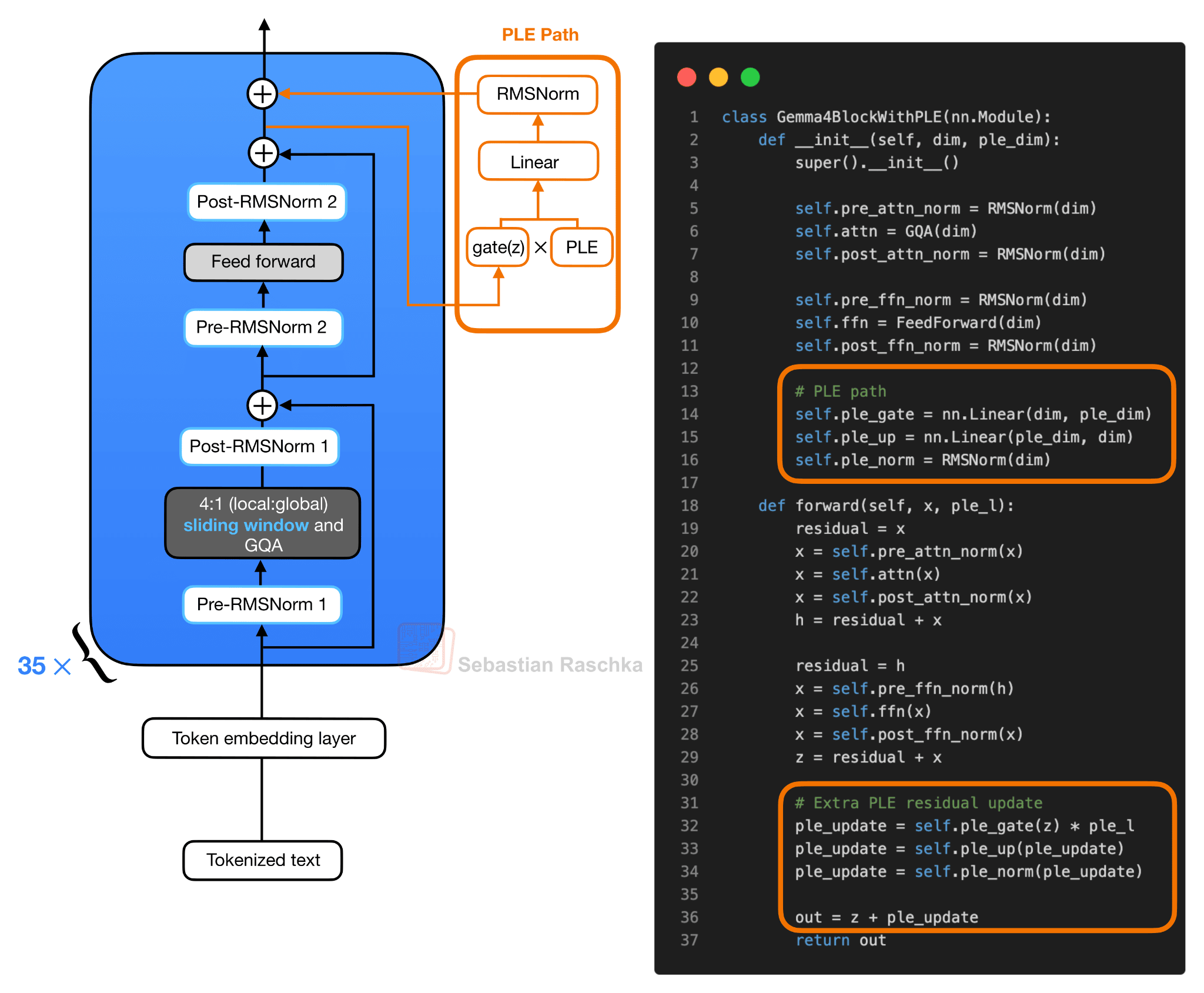
Conceptually, the new PLE path looks like this:

The PLE vectors themselves are prepared outside the repeated transformer blocks. In simplified form, there are two inputs to the PLE construction. First, the token IDs go through a per-layer embedding lookup. Second, the normal token embeddings go through a linear projection into the same packed PLE space. These two pieces are added, scaled, and reshaped into a tensor with one slice per layer. Note that each block then receives its own slice.

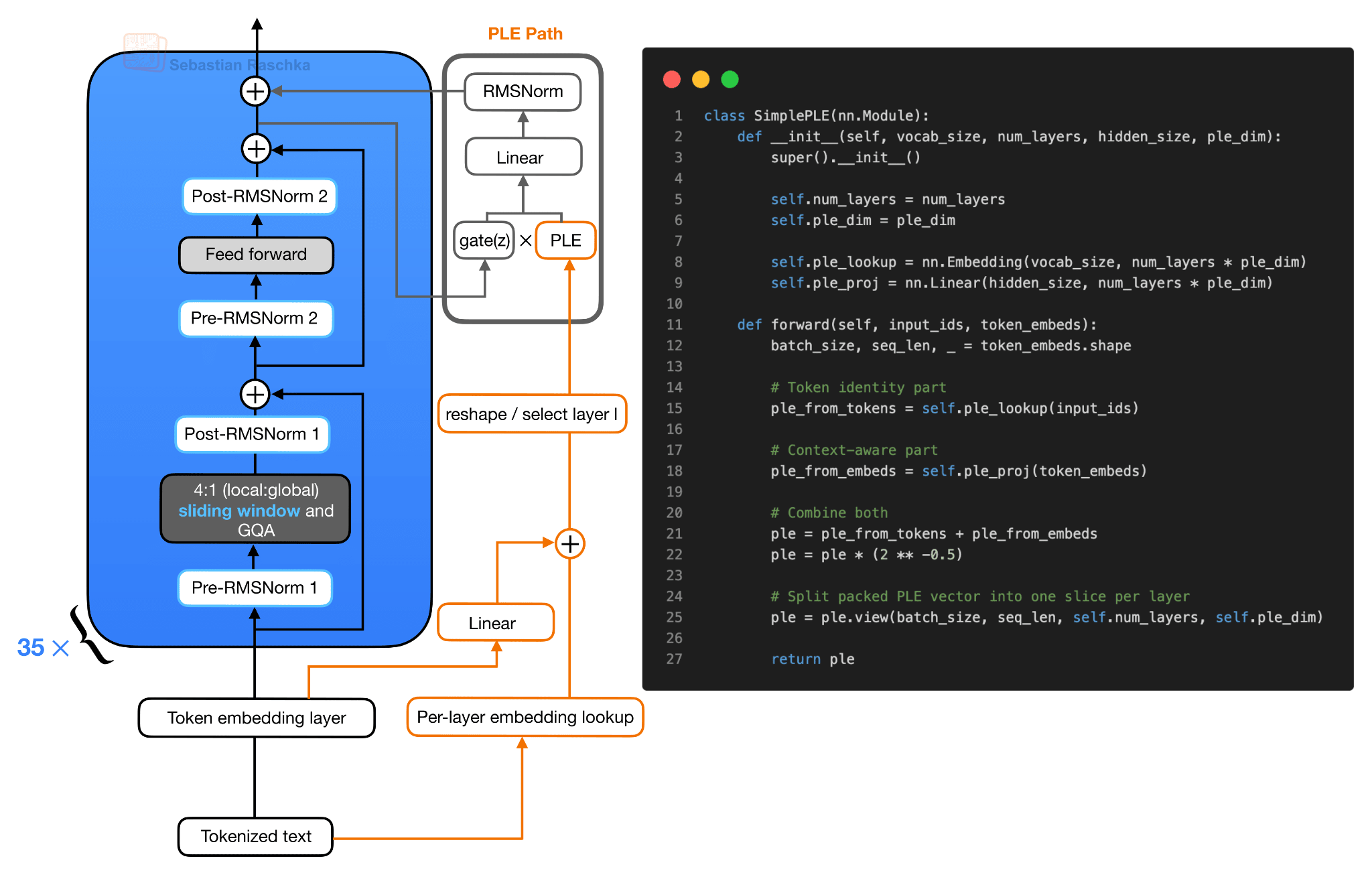
The important detail is that PLE does not give each transformer block a full independent copy of the normal token embedding layer. Instead, the per-layer embedding lookup is computed once. Then, as mentioned before, it gives each layer a small token-specific embedding slice (via “reshape / select layer l”.

So, for each input token, Gemma 4 prepares a packed PLE tensor that contains one small vector per decoder layer. Then, during the forward pass, layer l receives only its own slice (ple_l in the Gemma4WithPLEBlock in figure 6).

Inside the transformer block, the regular attention and feed-forward branches run as usual. First, the block computes the attention residual update. Then it computes the feed-forward residual update. After that second residual add, the resulting hidden state, which I denoted as z in the pseudocode in figure 6, is used to gate the layer-specific PLE vector. The gated PLE vector is projected back to the model hidden size, normalized, and added as one extra residual update.

So the useful mental model is that the transformer block still has the same main attention and feed-forward path, but Gemma 4 adds a small layer-specific token vector after the feed-forward branch. This increases representational capacity through embedding parameters and small projections. This adds computational overhead but avoids the cost of scaling the entire transformer stack to the larger parameter count.

But why PLEs? The simpler alternative would be to make the dense model smaller, using fewer layers, narrower hidden states, or smaller feed-forward networks. That would reduce memory and latency, but it also removes capacity from the parts of the model that do the main computation.

The PLE design keeps the expensive transformer blocks closer to the smaller “effective” size, while storing additional capacity in per-layer embedding tables. These are much cheaper to use than adding more attention or FFN weights, since they are mainly lookup-style parameters that can be cached.

Also, we have to take Google’s word here that this is an effective and worthwhile design choice. It would be interesting to see some comparison studies to see how this E2B design compares to a regular Gemma 4 2.3B model and a regular Gemma 4 5.1B model.

Also, in principle, PLE is not inherently limited to small models. We could attach per-layer embedding slices to larger models, too. However, larger models already have sufficient capacity where these extra embeddings may not help that much. Also, for larger models, we already use MoE designs as a trick to increase capacity while keeping the compute footprint smaller.

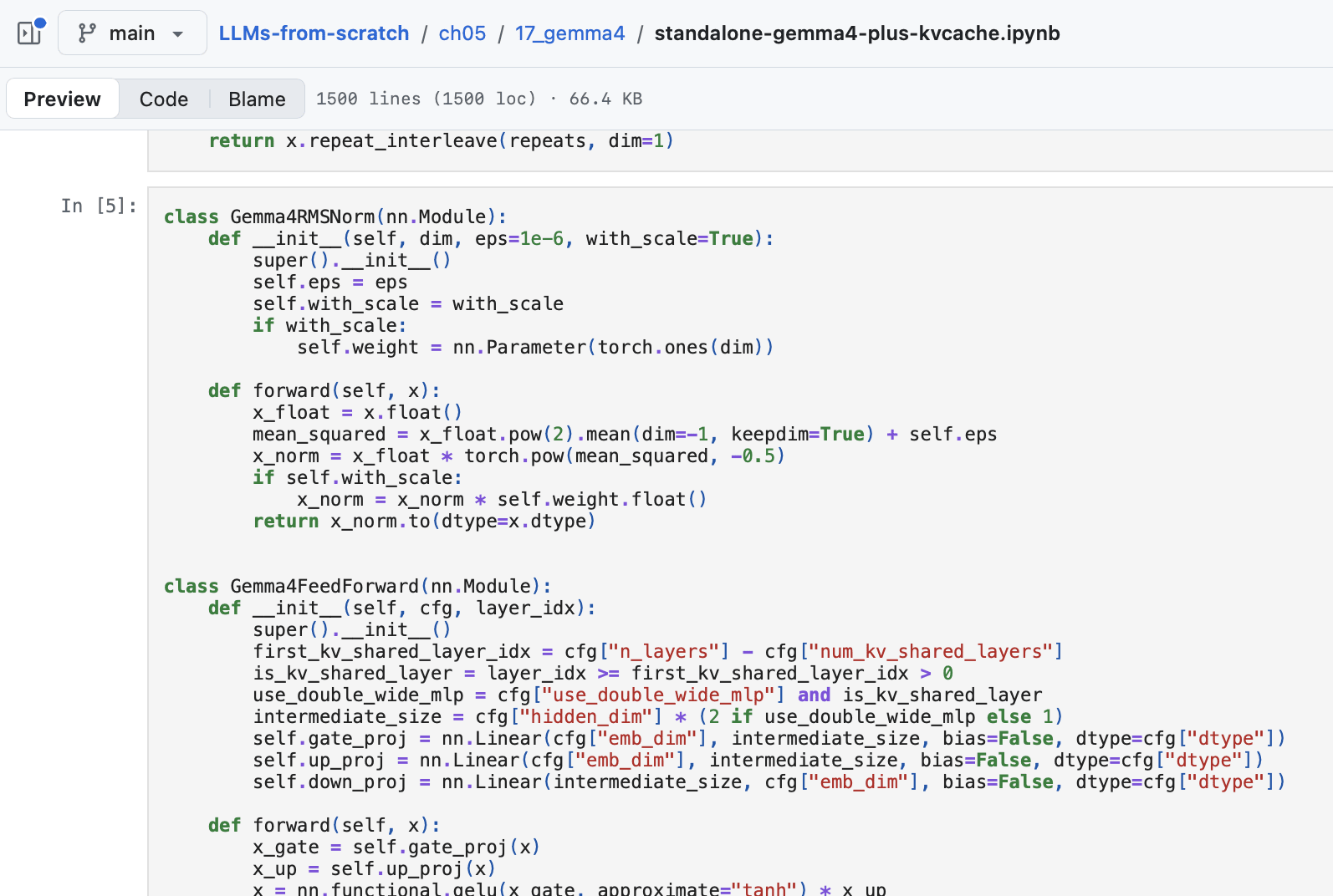
By the way, if you are interested in a relatively simple and readable code implementation, I implemented the Gemma 4 E2B and E4B models from scratch here.

3. Layer-Wise Attention Budgeting (Laguna XS.2)

Laguna is the first open-weight model by Poolside, a Europe-based company focused on training LLMs for coding applications. Several of my former colleagues joined Poolside in recent years, and they have a great team with lots of talent. It’s just nice to see more companies also releasing some of their models as open-weight variants.

Anyways, the Laguna XS.2 architecture depicted below looks very standard at first glance. However, one detail that I didn’t show (/try to cram into there) is a concept we can refer to as “Layer-wise attention budgeting”.

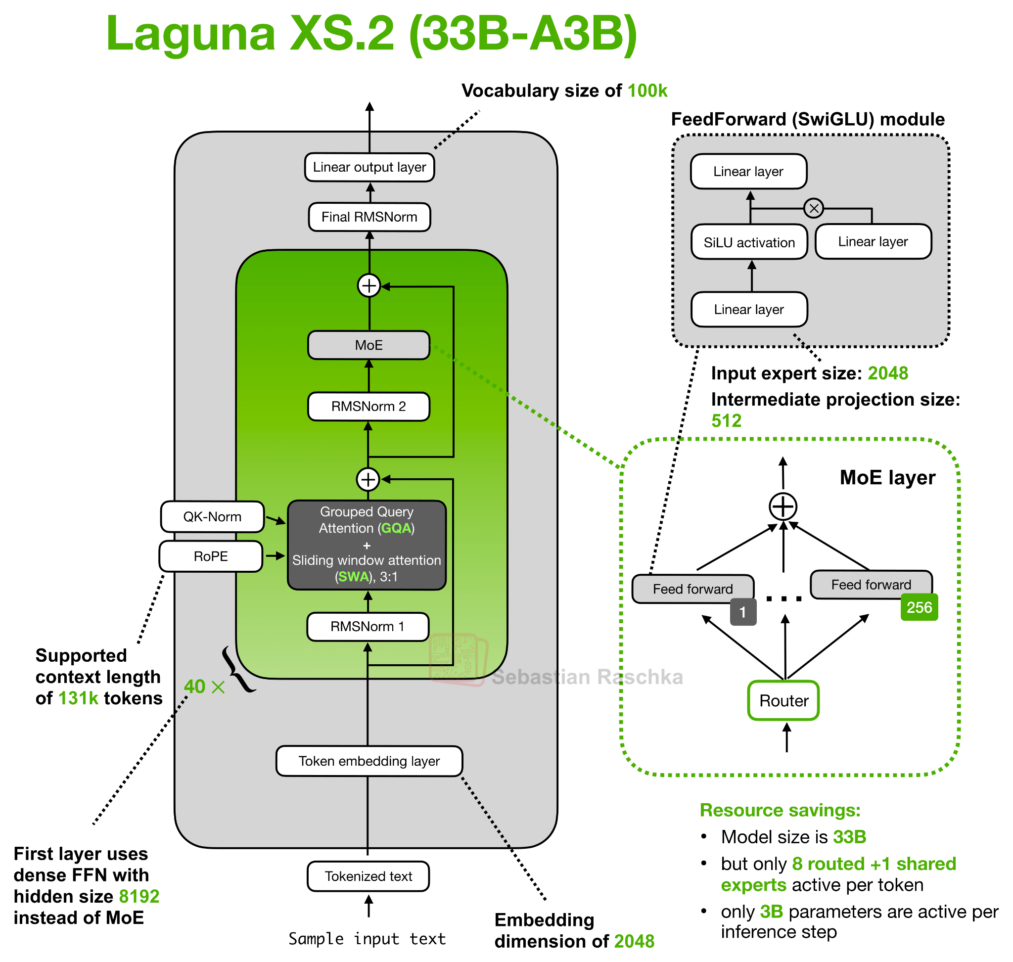
Part of the idea behind the attention budgeting here is that instead of giving every transformer layer the same full attention budget, Laguna XS.2 varies the attention cost by layer. It has 40 layers total, with 30 sliding-window attention layers and 10 global/full attention layers. As usual, the sliding-window layers only attend over a local window (here: 512 tokens), which keeps the KV cache and attention computation cheaper. The global layers are more expensive but preserve the ability to access all information in the context window.

This mixed sliding-window + global/full attention pattern is not unique to Laguna XS.2 and is used by many other architectures (including Gemma 4).

But what’s new is the use of per-layer query-head counts. For instance, the Hugging Face model hub config.json includes a num_attention_heads_per_layer setting, so layers can have different numbers of query heads while keeping the KV cache shape compatible.

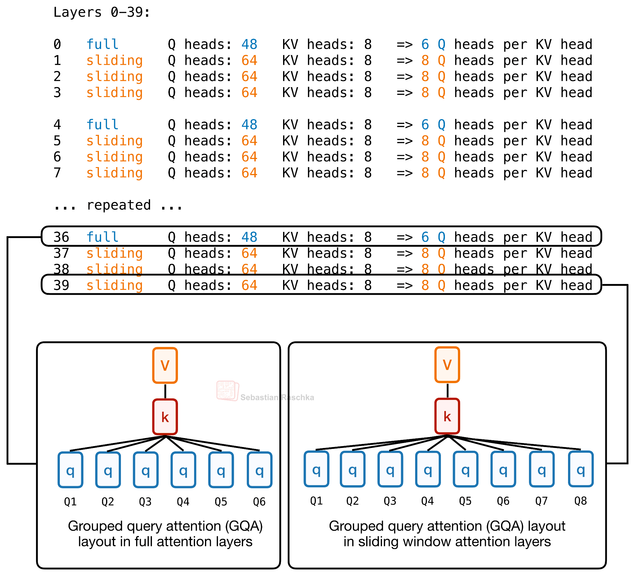
So Laguna XS.2 gives more query heads to sliding-window layers and fewer query heads to global layers, while keeping the KV heads fixed at 8. That is the actual layer-wise head budgeting in the config.

Laguna XS.2 is one of the most prominent recent examples of this per-layer query-head budgeting in a production-style open model. But the broader idea of varying model capacity by layer goes back to (at least) Apple’s 2024 OpenELM.

And again, what’s the point of such a design? Similar to KV-sharing, the point is to spend attention capacity where it is most useful, instead of giving every layer the same budget. Specifically, full-attention layers are expensive because they look across the whole context, so Laguna gives them fewer query heads compared to sliding window attention modules.

(Besides, another smaller implementation detail is that Laguna also applies per-head attention-output gating; this is somewhat similar to Qwen3-Next and others, which I also omit here since I covered it in earlier articles.)

4. Compressed Convolutional Attention (ZAYA1-8B)

Similar to Laguna, ZAYA1-8B is another new player on the open-weight market. It is developed by Zyphra, and one of the interesting details around the release is that the model was trained on AMD GPUs rather than the more common NVIDIA GPU (or Google TPU) setup.

The main architecture detail, though, is Compressed Convolutional Attention (CCA), used together with grouped-query attention. Unlike MLA-style designs that mainly use a latent representation as a compact KV cache format, CCA performs the attention operation directly in the compressed latent space, but more on that later.

(Sidenote: the ZAYA1-8B config.json lists 80 alternating layer entries rather than 40 conventional transformer blocks. These entries alternate between CCA/GQA attention and MoE feed-forward layers. But for the architecture figure, it is more convenient to visualize this as 40 repeated attention + MoE pairs, which is conceptually equivalent.)

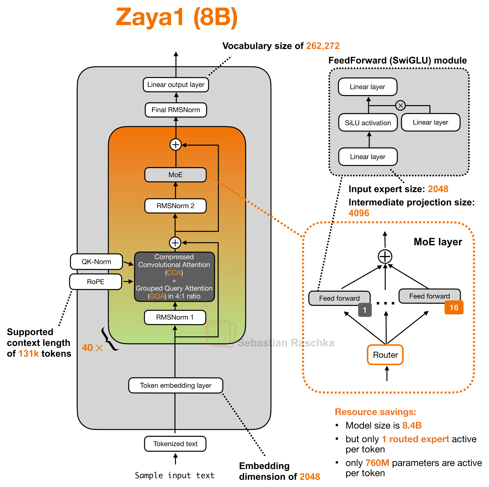
As hinted at in the figure above, ZAYA1-8B uses Compressed Convolutional Attention (CCA) together with a 4:1 GQA layout. The key point is that its attention block is built around CCA rather than a standard sliding-window attention block.

What is Compressed Convolutional Attention?

I would say CCA is related in spirit to Multi-head Latent Attention (MLA) in DeepSeek’s models, since both introduce a compressed latent representation into the attention block. However, they use that latent space differently. MLA mainly uses the latent representation to reduce the KV cache. In MLA, the KV tensors are stored compactly and then projected into the attention-head space for the actual attention computation.

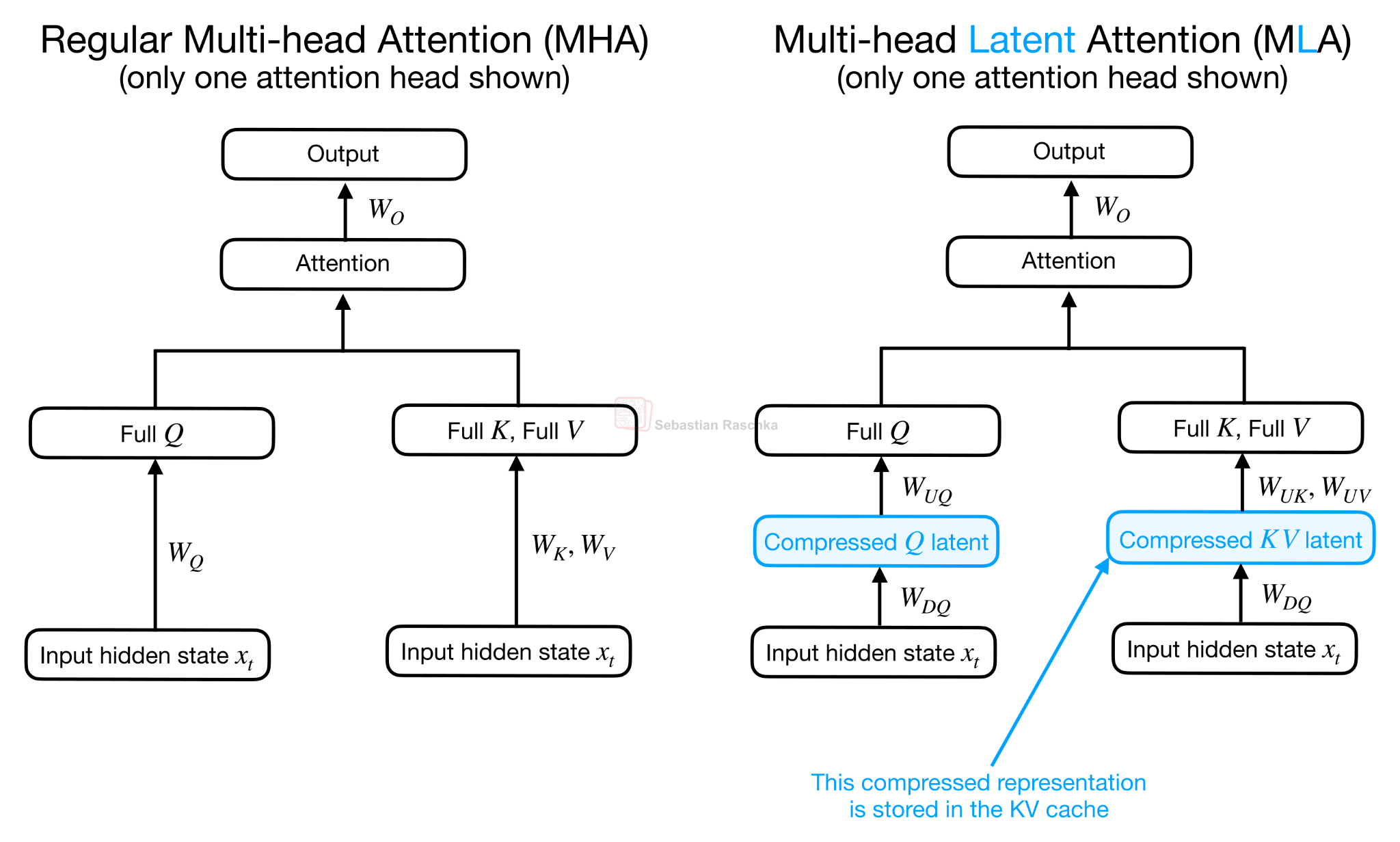
CCA compresses Q, K, and V and performs the attention operation directly in the compressed latent space. This is why CCA can reduce not only KV cache size, but also attention FLOPs during prefill and training.

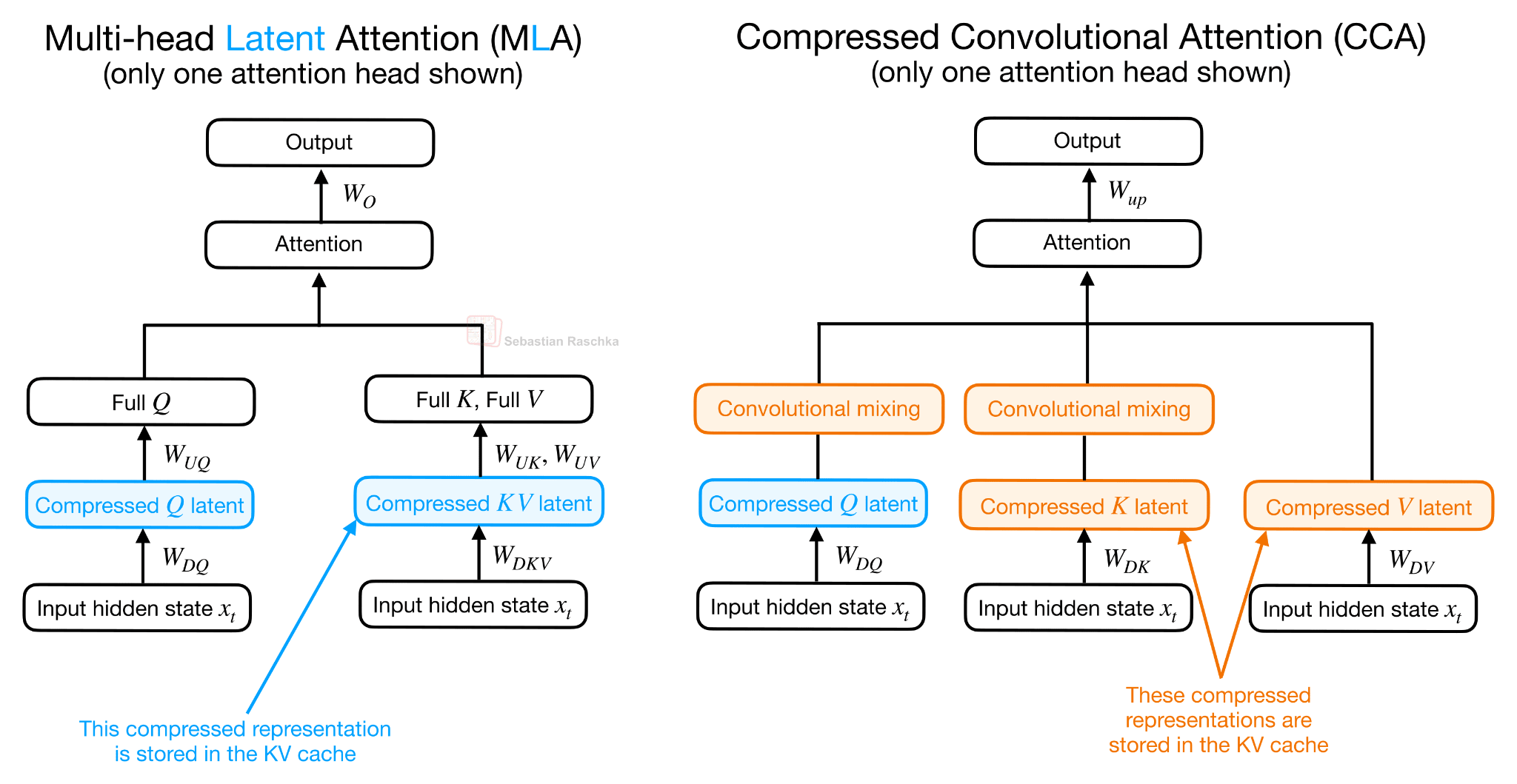
As Figure 13 above illustrates, in CCA, the compressed, latent representations enter the attention mechanism directly, and the resulting compressed attention vector is then up-projected.

Note that this is called Compressed Convolutional Attention, not just Compressed Attention, since there is an additional convolutional mixing happening on the latent K and Q representations. The convolutional mixing part is not shown in Figure 12, because it would have been too crammed, but it’s relatively straightforward.

As hinted at in Figure 12, the convolutional mixing happens directly on the compressed Q and K tensors. The point is that compression makes Q, K, and V narrower, which saves compute and cache, but it can also make attention less expressive. The convolutions are a cheap way to give the compressed Q and K vectors more local context before they are used to compute attention scores. (The convolutional mixing is only applied to Q and K, not V, because Q and K determine the attention scores, while V represents the content that gets averaged via these scores).

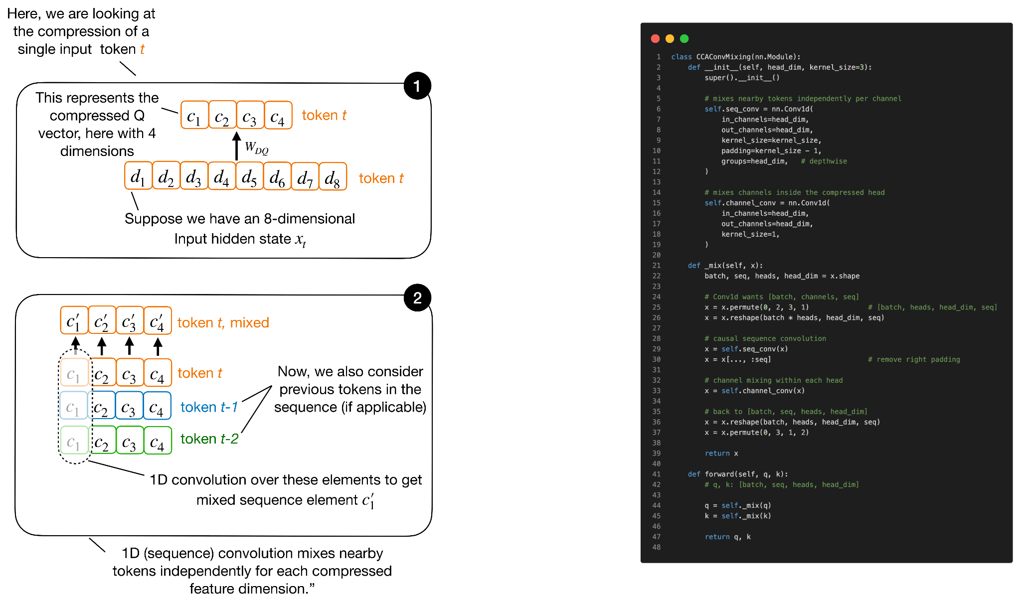
Next to the sequence mixing shown in Figure 13, there is also a channel mixing component. It’s in principle similar though, so I am omitting the illustration.

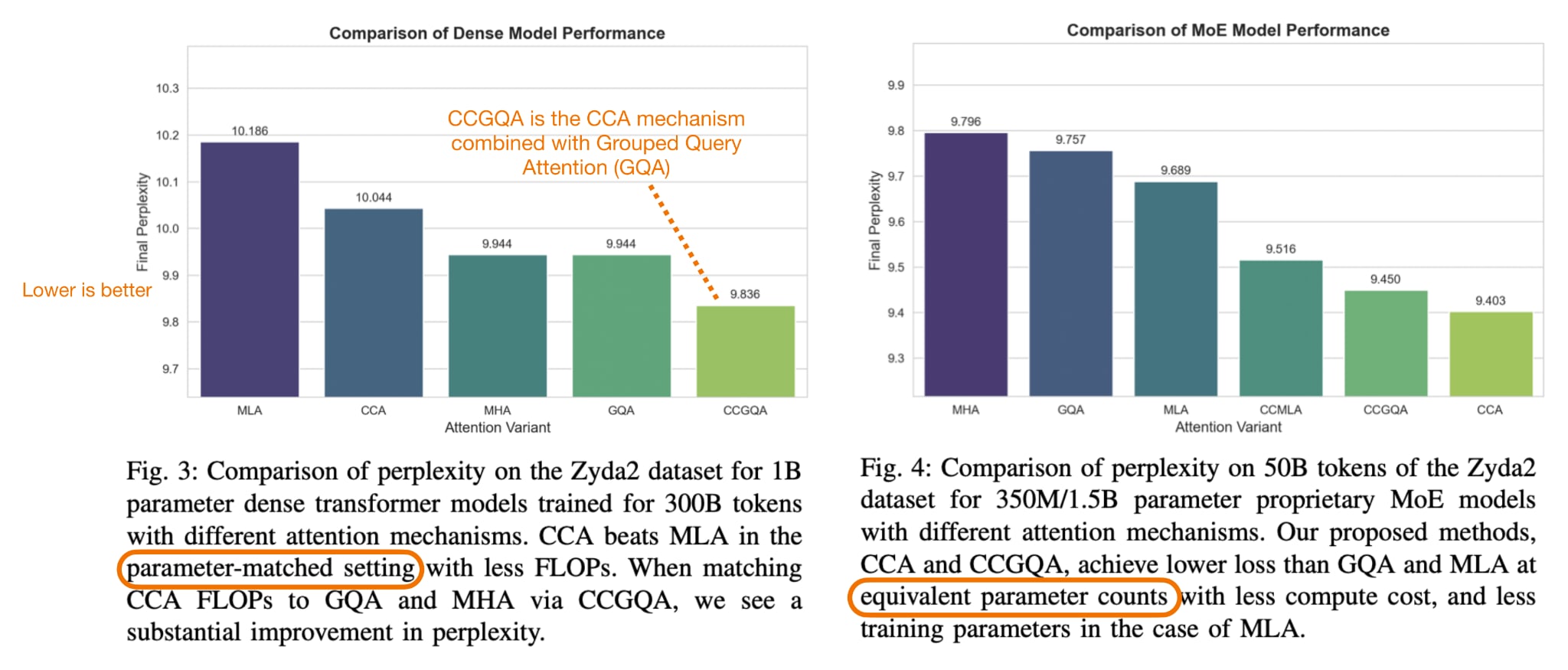
CCA appears to be a Zyphra-introduced attention mechanism that predates the ZAYA1-8B technical report. The standalone CCA paper, Compressed Convolutional Attention: Efficient Attention in a Compressed Latent Space, was first posted in October 2025 and explicitly introduces CCA. ZAYA1-8B then uses this mechanism as one of the core pieces.

But the question is, “is it better than MLA”? According to the CCA paper’s own experiments, yes, they report CCA outperforming MLA under comparable compression settings.

Overall, the interesting part here is really the new attention mechanism. The model also uses a pretty extreme (= very sparse) MoE setup, with only one routed expert active per token, but that part is more familiar. CCA is more unusual because it performs the attention operation directly in a compressed latent space, and then uses convolutional mixing on the compressed Q and K representations to make this compressed attention less limiting. So, in short, ZAYA1-8B is not only trying to save compute in the feed-forward layers, but also in the attention mechanism itself.

5. CSA/HCA, mHC, and Compressed Attention Caches (DeepSeek V4)

DeepSeek V4 was the biggest release of the year so far, both in terms of hype and model size. Interestingly, DeepSeek V4-Pro is also the most parameter-sparse MoE among the models in the table below, measured by active-parameter share, as summarized in the table below.

Caveat: active parameter share is only one lens. It does not capture KV cache size, attention pattern, context length, routing overhead, hardware efficiency, or training quality. But it is a helpful, quick check when comparing sparse models.

There’s a lot to say about DeepSeek V4, but since it’s been all over the news already, and to stay on topic regarding architecture tweaks, I will focus on the two most relevant parts that are new compared to previous architectures:

1. mHC for a wider residual pathway,

2. CSA/HCA for long-context attention compression and sparsity

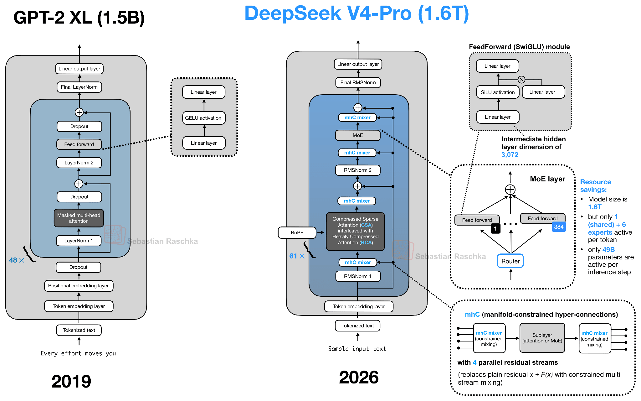
Looking at the DeepSeek V4 architecture drawing below, there seems to be a lot going on. The useful way to read it is to separate the residual-path change, mHC, from the attention-path changes, CSA/HCA, and compressed attention caches.

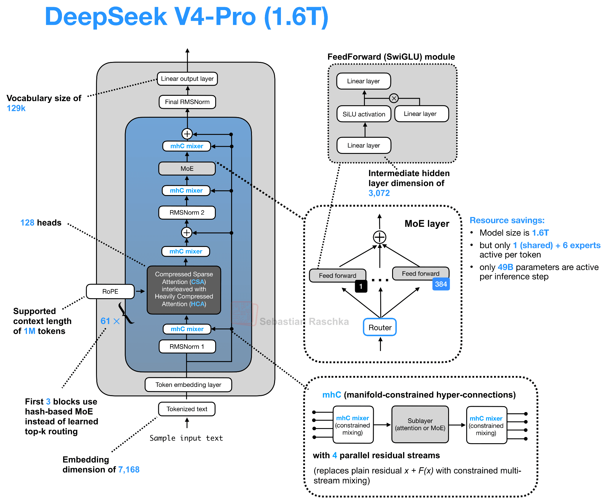
5.1 Manifold-Constrained Hyper-Connections (mHC)

Let’s start with the mHC component of DeepSeek V4. This goes back to a research paper that the DeepSeek team shared last year (31 Dec 2025, mHC: Manifold-Constrained Hyper-Connections). However, in this paper, the technique was only tested on an experimental 27B scale model. Now, we see it in their flagship release, which is a good sign that this idea actually works well in production.

The main idea behind mHC here is to modernize the design of the residual connections inside the transformer block, which is refreshing, because architecture tweaks are usually focused on the attention mechanism, normalization layer placement, and MoE parts.

Now, mHC is based on previous work on hyper-connections (see Hyper-connections by Zhu et al., 2024), which we should briefly discuss first. Hyper-connections essentially modify the single residual stream inside the transformer block by replacing it with several parallel residual streams and learned mappings between them.

(For those new to residual connections, I made a video on residual neural networks many years ago, where I explained the general mechanism.)

The idea behind hyper-connections is to widen the residual stream. We can think of this as keeping several parallel residual streams, with an additional Res Mapping linear transformation that mixes them across layers. Since the Attention or MoE layer itself still operates on the normal hidden size, hyper-connections also add a Pre Mapping that combines the parallel residual streams into one normal hidden vector for the layer, and a Post Mapping that distributes the layer output back across the parallel residual streams. This is visually summarized in the figure below.

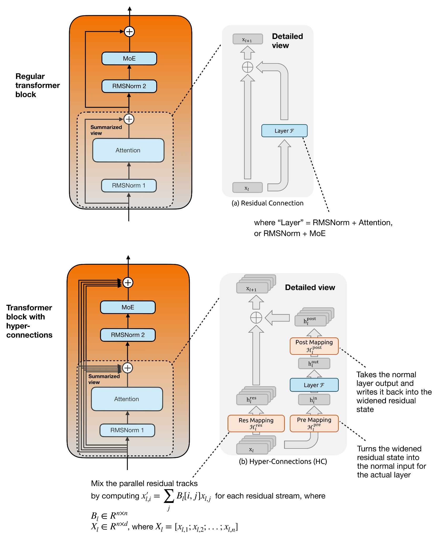
The figure below focuses on the attention-layer portion of the transformer block, but the same concept applies to the second residual branch around the MoE layer.

The purpose of hyper-connections is to make the residual pathway more expressive without making the actual Attention or MoE layer wider. This is only mildly more expensive in FLOPs because the extra mappings operate over the small residual-stream axis, for example, n = 4 in DeepSeek V4, not over a huge hidden dimension.

In the original hyper-connections paper, the 7B OLMo MoE experiment goes from 13.36G to 13.38G FLOPs per token, which is basically unchanged. In terms of reported gains, there were modest (but consistent) improvements, as shown in the figure below.

(However, only looking at FLOPs is a bit simplistic. The widened residual state still has to be stored, moved through memory, mixed, etc. So the practical overhead can come more from memory traffic and implementation complexity than from arithmetic, which is not explicitly measured. However, given that DeepSeek V4 is all about efficiency, it seems to be a worthwhile addition.)

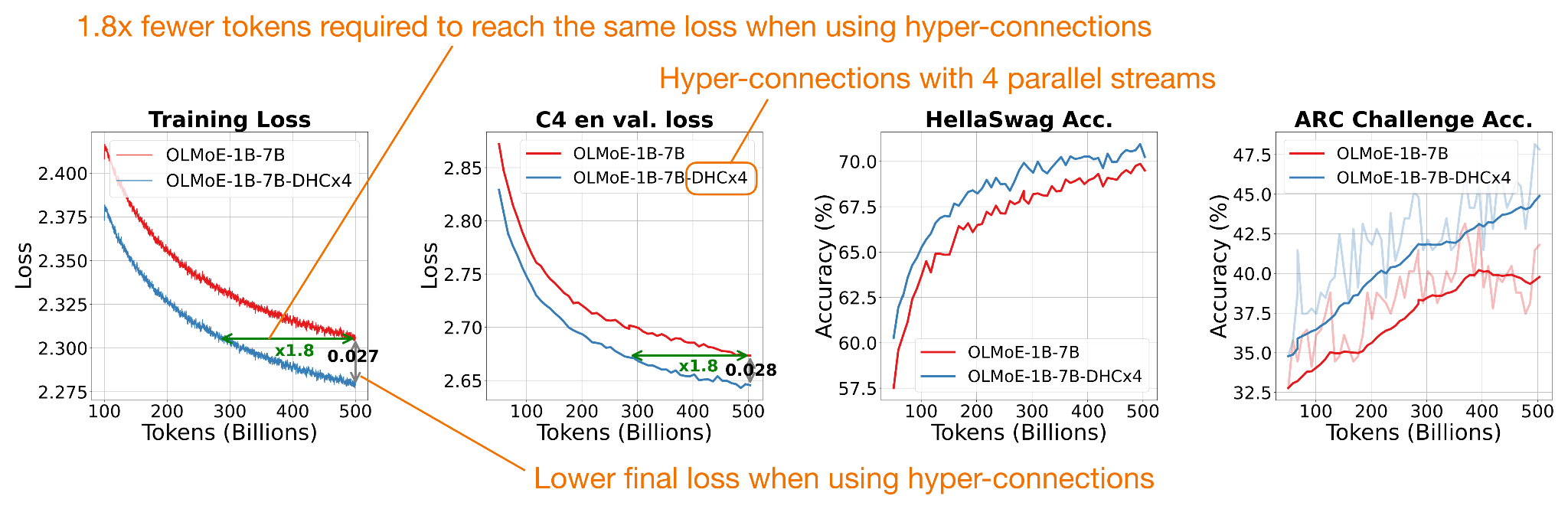
Also, as shown in the figure above, metrics reached the baseline’s performance using roughly half the training tokens.

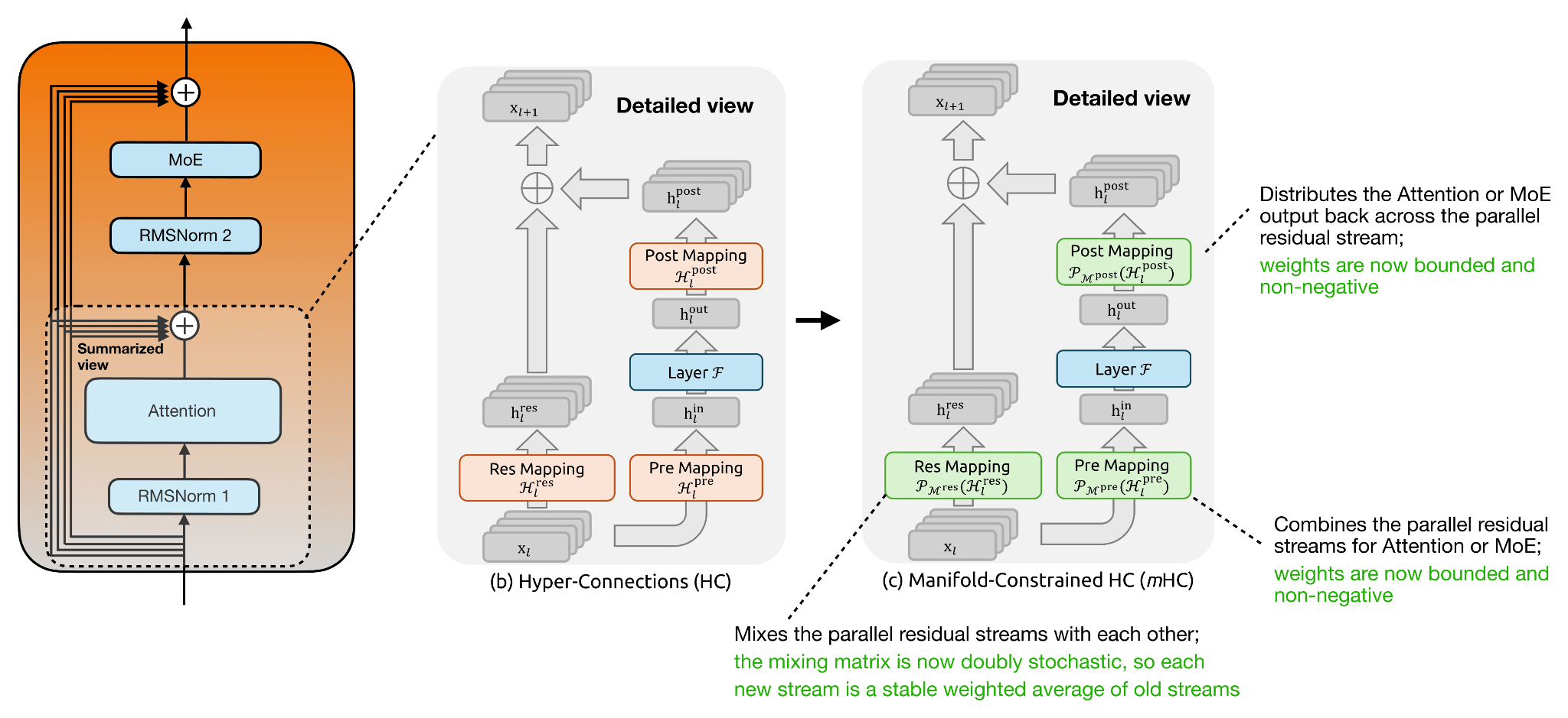
The main change from regular hyper-connections (HC) to manifold-constrained hyper-connections (mHC) is that the mappings are no longer left unconstrained. In regular HC, the Res Mapping is a learned matrix that mixes the parallel residual streams, but stacking many such matrices can amplify or shrink signals unpredictably.

In mHC, this residual mapping is projected onto the manifold of doubly stochastic matrices, meaning all entries are non-negative and each row and column sums to 1. This makes the residual mixing behave more like a stable redistribution of information across streams. The Pre Mapping and Post Mapping are also constrained to be non-negative and bounded, which avoids cancellation when reading from and writing back into the widened residual state. In short, mHC keeps the richer residual mixing of HC, but adds constraints so it scales more safely, which becomes more relevant for larger (deeper) models.

Otherwise, the main idea of using parallel residual streams remains, as shown in the figure below.

In the mHC paper, using a 27B parameter model for the experiments, the DeepSeek team’s optimized implementation (with fusion, recomputation, and pipeline scheduling) adds only 6.7% additional training time overhead for 4 residual streams (n = 4) throughout all transformer blocks compared to the single-stream baseline.

To sum up this section, HC/mHC changes how information is carried around these layers by replacing the single residual stream with several interacting residual streams, with the additional stability constraints added in mHC, while adding minimal compute overhead. Also, it pairs well with the CSA/HCA attention changes, which modify other parts of the transformer block, which I will discuss below.

5.2 Compressed Attention via CSA and HCA

The other major DeepSeek V4 architecture change is on the attention side. Again, the motivation is that at very long context lengths, attention becomes expensive not only because of the attention score computation, but also because the KV cache grows with the sequence length. DeepSeek V4 addresses this issue with a hybrid of two compressed-attention mechanisms, Compressed Sparse Attention (CSA) and Heavily Compressed Attention (HCA).

For a refresher, I recommend checking out my previous “A Visual Guide to Attention Variants in Modern LLMs” article, which covers Multi-head Latent Attention (MLA) and DeepSeek Sparse Attention (DSA), among others.

The first thing to note is that CSA/HCA in DeepSeek V4 is a different kind of compression than the MLA-style compression used in DeepSeek V2/V3. Where MLA mainly compresses the per-token KV representation, CSA and HCA compress along the sequence dimension. So, instead of keeping one full (or compressed) KV entry for every previous token, they summarize groups of tokens into fewer compressed KV entries. Consequently, the cache gets shorter. DeepSeek V4 also uses compact compressed entries and shared-KV attention, but the main distinction from MLA is the sequence-length compression. This is illustrated in the figure below.

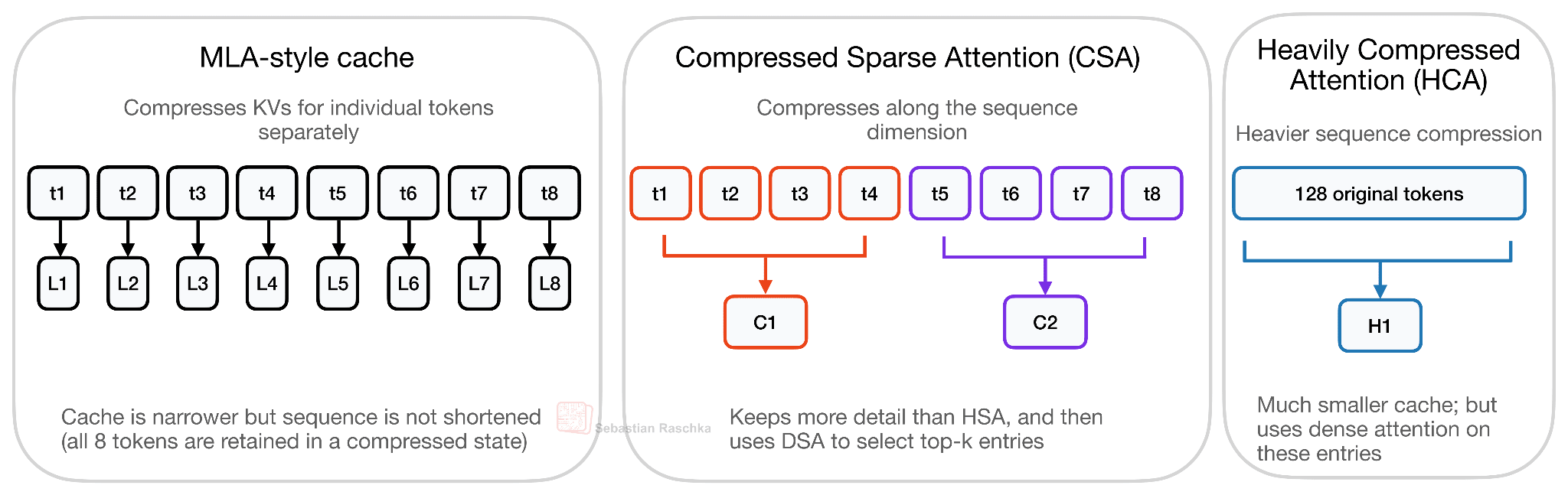
The quality tradeoff for CSA/HCA is also different from MLA. As shown in the figure above, MLA compresses the representation stored for each token, but it still keeps one latent KV entry per token. CSA and especially HCA go further by reducing the number of sequence entries themselves, so the model gives up some token-level info in exchange for much lower long-context cost.

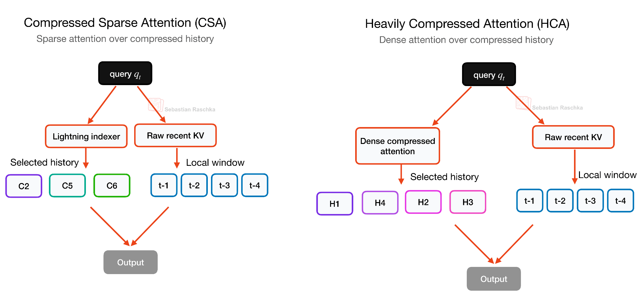
Again, it’s all about reducing long-context cost, but this trade-off can hurt modeling quality if the compression is too strong, which is why DeepSeek V4 does not rely on one compression scheme alone but alternates between CSA and HCA. CSA uses a milder compression rate and a DeepSeek Sparse Attention (DSA)-style selector, HCA uses much heavier compression for cheaper global coverage, and both keep a local sliding-window branch for recent uncompressed tokens. This sparse selection in CSA builds on DeepSeek Sparse Attention (DSA), which I discussed in more detail in my earlier DeepSeek V3.2 write-up.

HCA is the more aggressive variant of the two. It compresses every 128 tokens into one compressed KV entry, but then uses dense attention over those heavily compressed entries. In other words, CSA keeps more details but uses sparse selection, while HCA keeps far fewer entries and can afford dense attention over them, as illustrated in the figure below. This makes the two mechanisms somewhat complementary, which is why DeepSeek V4 interleaves CSA and HCA layers rather than using only one of them.

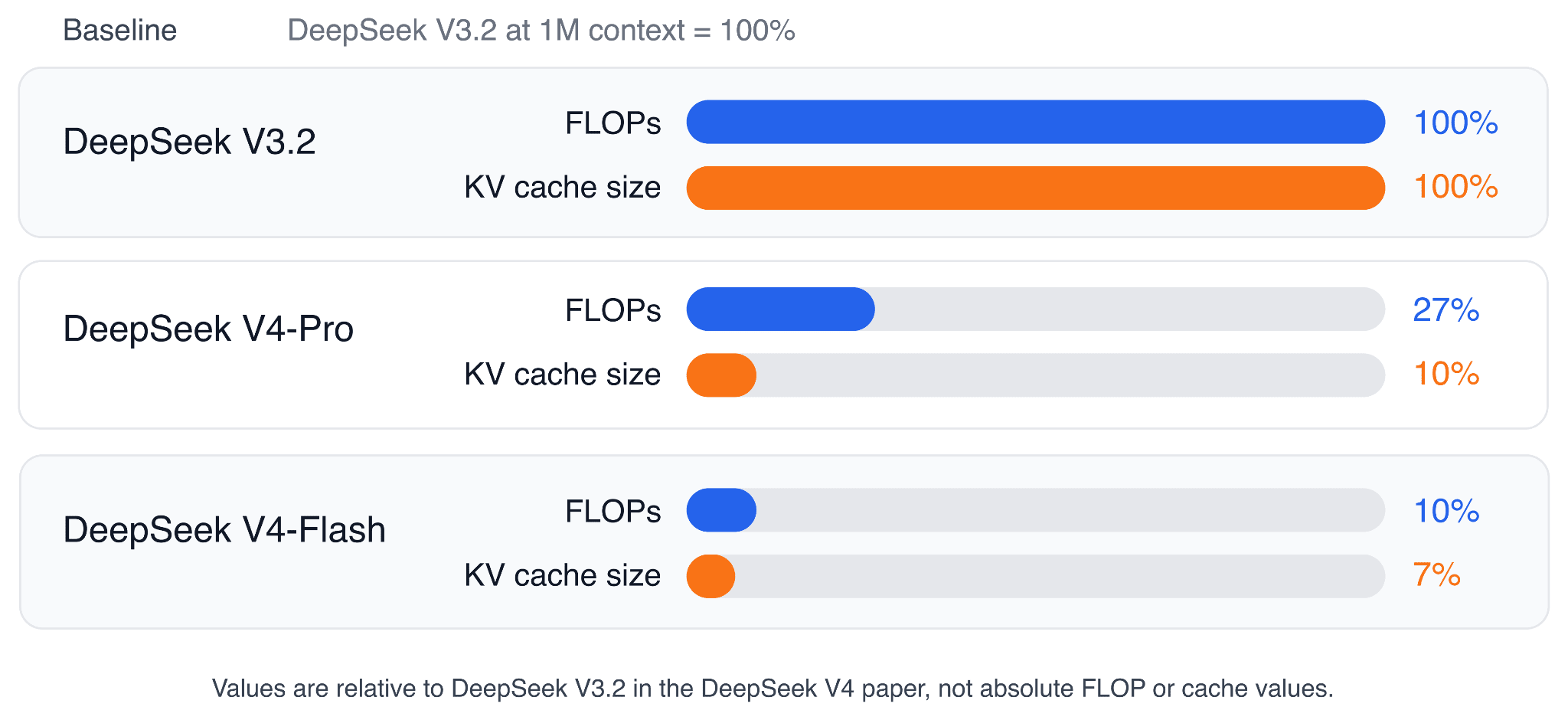
The DeepSeek V4 paper reports that, at a 1M-token context length, DeepSeek V4-Pro uses only 27% of the single-token inference FLOPs and 10% of the KV cache size compared with DeepSeek V3.2, which uses MLA and DeepSeek Sparse Attention (DSA). DeepSeek V4-Flash is even smaller, at 10% of the FLOPs and 7% of the KV cache size relative to DeepSeek V3.2.

By the way, I would not describe CSA/HCA as “better” than MLA in a general sense. CSA/HCA is a more aggressive long-context design. And it’s also more complicated for sure. Unfortunately, there is no ablation study in the paper. But overall, the paper reports strong overall modeling results, including DeepSeek V4-Flash-Base outperforming DeepSeek V3.2-Base on a majority of base-model benchmarks and strong 1M-token retrieval results, but these results are for the full DeepSeek V4 recipe, which also includes better data, Muon-based optimization, mHC, precision/storage optimizations, and training/inference-system changes.

Personally, for now, I would treat CSA/HCA as an efficiency-focused long-context design that appears to preserve modeling quality well in their large flagship model(s) but not necessarily universally better than MLA.

6. Conclusion

Overall, the interesting pattern this year is that most new open-weight models try to make long-context inference cheaper without just shrinking the model in terms of total parameters. For instance,

• Gemma 4 reduces KV-cache memory with cross-layer KV sharing and adds capacity via per-layer embeddings.

• Laguna XS.2 tweaks how much attention capacity each layer gets.

• ZAYA1-8B moves attention into a compressed latent space.

• DeepSeek V4 adds constrained residual-stream mixing and compressed long-context attention.

All of these tweaks add more complexity, which seems to be where LLM architecture is going right now.

My main takeaway is that the transformer block is still changing, but in fairly targeted ways. The basic recipe is still based on the original GPT decoder-only transformer architecture, but many parts are upgraded or replaced, and they get more specialized for longer contexts and more efficient inference, whereas the qualitative modeling performance seems largely driven by data quality (and quantity) and training recipes.

The question many of you asked me in the past is centered on when (or if) transformers are being replaced with something else. Of course, there are other designs like diffusion models, but transformers remain the status quo for state-of-the-art architecture releases.

However, with each increasing yearly release quarter, we get more and more tweaks. While it was possible to implement a basic transformer block in perhaps 50-100 lines of PyTorch code, these tweaks (esp. around the attention variants) probably 10x the code complexity. This is not an inherently bad thing as these tweaks reduce (not increase) runtime costs. However, it’s becoming increasingly difficult to gain a clear understanding of the individual components and their interactions.

For instance, I am fairly certain that someone who is diving into LLM architectures for the first time will be totally overwhelmed when seeing the DeepSeek V4 source code. However, by starting with the original decoder-style LLM (GPT/GPT-2) and then gradually adding / learning about these new components one at a time, we can keep the learning effort manageable. The moral of the story, I guess, is to keep learning, one architecture at a time :).

By the way, I am very excited to share that I finished writing Build A Reasoning Model (From Scratch) and all chapters are in early access now. The publisher and I worked hard on the final layouts in the past month, and it’s going to be send to the printer this week. (Good news: the print version will be in color this time!)

This is probably my most ambitious book so far. I spent about 1.5 years writing it, and a large number of experiments went into it. It is also probably the book I worked hardest on in terms of time, effort, and polish, and I hope you’ll enjoy it.

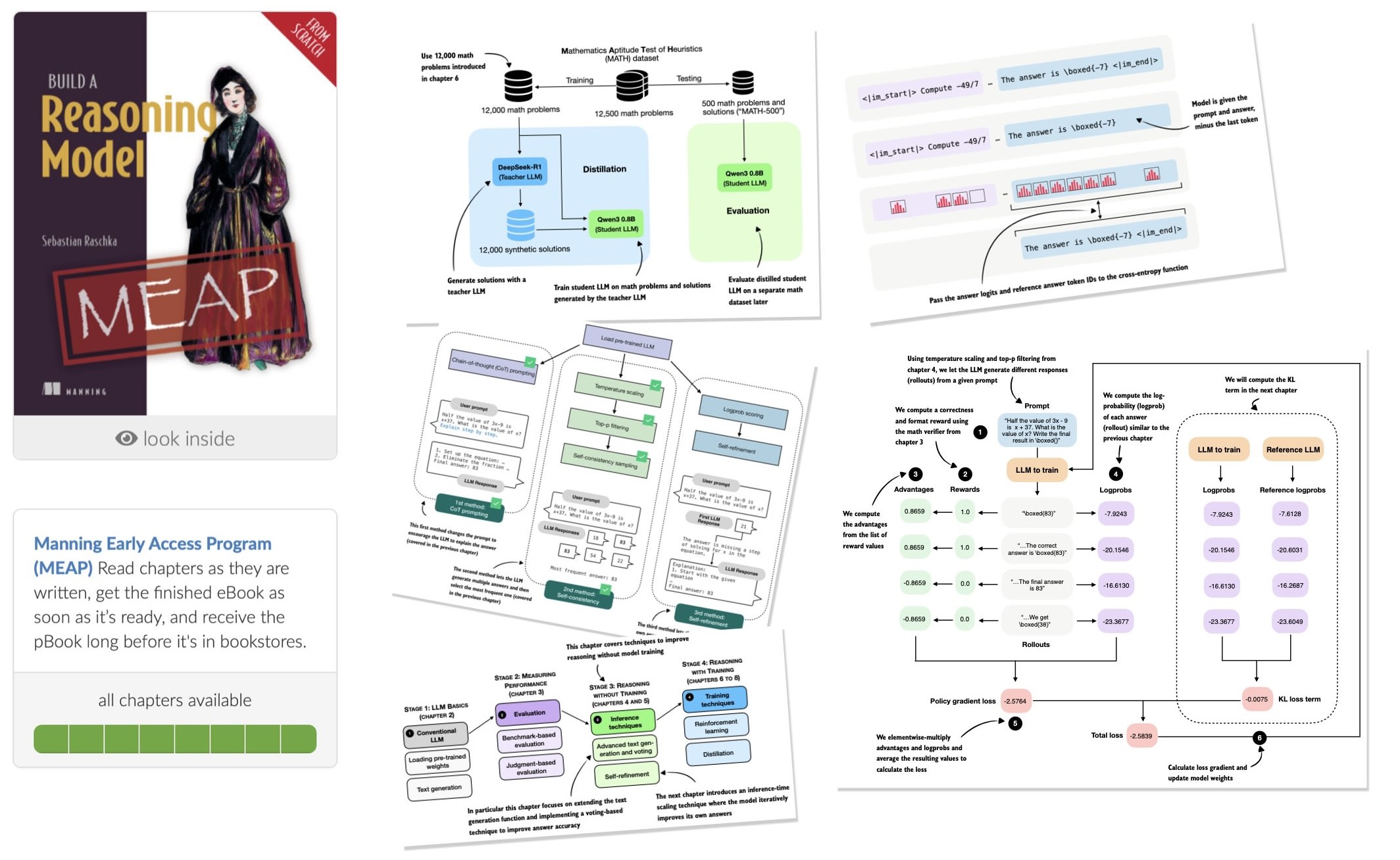
The main topics are

• evaluating reasoning models

• inference-time scaling

• self-refinement

• reinforcement learning

• distillation

There is a lot of discussion around “reasoning” in LLMs, and I think the best way to understand what it really means in the context of LLMs is to implement one from scratch!

• Amazon (pre-order of Kindle ebook and print paperback)

• Manning (complete book in early access, pre-final layout, 528 pages)